
Omega Ratio Threshold Partition (LPM1): Full-Distribution Skew & Kurtosis Math
Unlike Sharpe (2 moments) or Sortino (LPM2), the Keating-Shadwick Omega Ratio partitions the entire empirical return CDF around threshold tau, embedding every higher moment automatically.
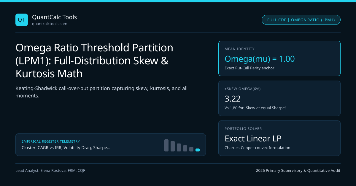
Mean-variance Sharpe ratios ignore third and fourth moments entirely, and even Cornish-Fisher expansions truncate after fourth-order kurtosis—becoming unstable on bimodal or option-linked return distributions (such as structured notes, merger arbitrage, or tail-hedged equities). Introduced by Con Keating and William Shadwick (2002), the Omega Ratio $\Omega(\tau)$ eliminates parametric moment truncation altogether: by partitioning the entire cumulative distribution function (CDF) $F(R)$ at an investor-chosen return threshold $\tau$, Omega incorporates mean, variance, skewness, kurtosis, and every higher-order moment exactly as observed in the empirical data! Audit return distributions with our Omega & Calmar Engine, Sharpe & Sortino Calculator, and CAGR, IRR & Drawdown Hub.
Three Equivalent Mathematical Representations: CDF Area, $LPM_1$, and Call-Over-Put Parity#
Let $F(x) = \mathbb{P}(R \le x)$ be the cumulative return distribution on $[a, b]$. Integrating by parts proves that Keating & Shadwick's upper-to-lower CDF area ratio equals expected upside gain divided by expected downside loss ($UPM1(\tau) / LPM1(\tau)$)—which in derivatives pricing is literally the undiscounted payoff of a European Call option struck at $\tau$ divided by a European Put option struck at $\tau$!
- 1. CDF Integral Form : Omega(tau) = [ Integral{tau..b} (1 - F(x)) dx ] / [ Integral{a..tau} F(x) dx ]
- 2. Call / Put LPM_1 Form : Omega(tau) = E[ max(0, R - tau) ] / E[ max(0, tau - R) ]
- 3. Put-Call Parity Link : Since E[max(0, R - tau)] - E[max(0, tau - R)] = E[R] - tau:
- Omega(tau) = 1 + ( E[R] - tau ) / LPM_1(tau)
- Exact Discrete Sample Estimator (N Period Returns R1..RN, No Histogram Binning Required!):
- Omegahat(tau) = [ Sum{t=1..N} max(0, Rt - tau) ] / [ Sum{t=1..N} max(0, tau - R_t) ]
- Worked Bimodal Skewness Test (N = 10 Years, Both Funds Have E[R] = +10.0% and Sigma = 18.97%!):
- Fund PosSkew (Trend/VC) : Nine years of +4.0% and ONE breakout year of +64.0% (Mean = 10.0%, Vol = 18.97%)
- Fund NegSkew (Short Put): Nine years of +16.0% and ONE crash year of -44.0% (Mean = 10.0%, Vol = 18.97%)
- > At Threshold tau = +6.0% Hurdle:
- Fund PosSkew: Gains above 6% = 1(58%) = 58% | Losses below 6% = 9(2%) = 18% => Omega(6%) = 58 / 18 = 3.22!
- Fund NegSkew: Gains above 6% = 9(10%) = 90% | Losses below 6% = 1(50%) = 50% => Omega(6%) = 90 / 50 = 1.80!
- (Sharpe TIED both funds at 0.290, yet Omega(6%) ranks PosSkew +78.9% superior due to crash protection!)
Look at the elegance of Form 3 (Omega(tau) = 1 + (E[R] - tau) / LPM_1(tau)):
- At $\tau = \mathbb{E}[R]$ (threshold equal to the portfolio's arithmetic mean return), $\mathbb{E}[R] - \tau = 0$, so $\Omega(\mathbb{E}[R]) = 1.000$ identically for EVERY distribution in the universe!
- For $\tau < \mathbb{E}[R]$, $\Omega(\tau) > 1$; for $\tau > \mathbb{E}[R]$, $\Omega(\tau) < 1$; and $\Omega(\tau)$ is a strictly monotonically decreasing curve across $\tau$.
Why Plotting the Full $\Omega(\tau)$ Curve Reveals Regime Crossings#
Rather than evaluating $\Omega(\tau)$ at a single scalar point, institutional risk desks plot the Omega Curve $\ln \Omega(\tau)$ across a continuum of thresholds $\tau \in [-5\%, +15\%]$:
- At low thresholds ($\tau = -2\%$), $\Omega(-2\%)$ is dominated by left-tail catastrophe protection: strategies with hard stop-losses or protective Black-Scholes put overlays tower above short-volatility carry strategies.
- At high aggressive thresholds ($\tau = +12\%$), $\Omega(+12\%)$ measures right-tail lottery upside: concentrated venture or momentum sleeves overtake low-volatility defensive bond portfolios!
Stochastic Dominance & Lower-Partial-Moment Hierarchy (Sharpe, Omega, Sortino, Kappa)#
Map how partial moment order $\alpha \in \{1, 2, 3\}$ governs higher-moment capture and sub-hurdle crash aversion:
| Risk-Adjusted Metric | Lower Partial Moment Order | Higher Moments Captured | Risk Aversion Assumption (Fishburn) | Ranking Crossing Possible? |
|---|---|---|---|---|
| Sharpe Ratio | Two-sided $\sigma$ ($L_2$) | $1\text{st}$ & $2\text{nd}$ only | Quadratic utility / Elliptical dist | Fixed scalar |
| Omega Ratio ($\Omega(\tau)$) | $LPM_1(\tau)$ (Linear) | All moments ($1.. \infty$) | Risk-neutral below $\tau$ ($\alpha = 1$) | Yes across $\tau$ |
| Sortino Ratio | $LPM_2(\tau)$ (Quadratic) | Downside $2\text{nd}+$ | Strictly risk-averse below $\tau$ ($\alpha = 2$) | Yes across $\tau$ |
| Kappa-3 Ratio (Kaplan) | $LPM_3(\tau)$ (Cubic) | Extreme crash $3\text{rd}+$ | Hyper-sensitive to tail ruin ($\alpha = 3$) | Yes across $\tau$ |
Subtle Theoretical Caveat: $LPM1$ vs $LPM2$ Second-Order Stochastic Dominance#
While Keating & Shadwick popularized Omega for capturing all distribution moments, Kaplan & Knowles (2004) highlighted an important utility-theory nuance: because Omega's denominator $LPM1(\tau) = \mathbb{E}[\max(0, \tau - R)]$ weights losses linearly ($1\times$ a $-20\%$ crash equals $10\times$ a $-2\%$ dip!), maximizing $\Omega(\tau)$ alone does not enforce strict risk aversion within the loss region below $\tau$. By contrast, [Sortino's $LPM2(\tau)$](/guides/sortino-ratio-target-downside-semi-deviation-mar-denominator-math) squares losses ($20^2 = 400$ vs $10 \times 2^2 = 40$), guaranteeing Fishburn second-order stochastic dominance! Institutional allocators therefore inspect both $\Omega(\tau)$ and $\text{Sortino}(\tau)$ side-by-side.
Linear Programming Portfolio Optimization with Omega#
Unlike Sharpe or Sortino optimization (which require quadratic or non-linear solvers), Mausser, Saunders & Seco (2006) showed that maximizing portfolio $\Omega_p(\tau)$ over asset weights $w$ transforms via the Charnes-Cooper fractional-programming substitution into a fast, exact Linear Program (LP)! Pair Omega portfolio rankings with Calmar & Ulcer path-dependent ratios and Probabilistic / Deflated Sharpe significance tests, and inspect institutional analytics across rankings and Central Bank of Ireland UCITS disclosures.
Frequently asked questions
Why does the Omega Ratio always equal 1.0 when the threshold tau equals the sample mean return?
Any random variable satisfies the identity R - mu = max(0, R - mu) - max(0, mu - R). Taking expectations on both sides yields 0 = E[max(0, R - mu)] - E[max(0, mu - R)], so expected gains above the mean always equal expected shortfalls below the mean—making their ratio exactly 1.00!
How is the Omega Ratio related to the Sharpe Ratio if returns actually ARE Normally distributed?
For R ~ N(mu, sigma^2), letting z = (tau - mu) / sigma, closed-form Gaussian integration gives Omega(tau) = [phi(z) - z*(1 - Phi(z))] / [phi(z) + z*Phi(z)], which is a strictly monotonic one-to-one function of -z = (mu - tau)/sigma (the Sharpe ratio when tau = r_f)!
Should I annualize monthly returns before or after computing the Omega Ratio?
Never multiply Omega by sqrt(12)! Omega is a dimensionless gain-to-loss probability-weighted dollar ratio. Convert your annual hurdle tau_annual into a monthly threshold tau_m = (1 + tau_annual)^(1/12) - 1 and compute Omega(tau_m) directly on monthly returns (or rolling 12-month returns if capturing serial path effects).
What are Kaplan-Knowles Kappa Ratios and how do they connect Omega and Sortino?
Kaplan & Knowles (2004) unified downside performance ratios into Kappa_n(tau) = (E[R] - tau) / [LPM_n(tau)]^(1/n). Setting n = 1 yields Kappa_1(tau) = Omega(tau) - 1; setting n = 2 yields exact Sortino(tau); and setting n = 3 yields cubic crash-averse Kappa_3(tau)!
Publication record
- Published
- 13 November 2026
- Updated
- 14 November 2026
- Author
- Elena Rostova, FRM, CQF
- Review
- Review not recorded
- Automated fact check
- Passed in the stored pipeline record
- Source URLs
- 4 recorded
AI assistance recorded: anthropic/claude-opus-4.6. This field does not establish human review or source verification.
Academic & Institutional Attribution
Cite This Research & Embed Live Data Card
Standard academic & institutional research paper citation format.
Elena Rostova, FRM, CQF. (2026, November 14). Omega Ratio Threshold Partition (LPM1): Full-Distribution Skew & Kurtosis Math. QuantCalc Tools. https://quantcalctools.com/guides/omega-ratio-threshold-partition-lpm1-positive-skew-ranking-mathRelated Cagr Irr Drawdown Compounding & Institutional Briefings
Explore Cagr Irr Drawdown Compounding Hub (20) →Cagr Irr Drawdown Compounding
CAGR vs IRR, Volatility Drag, Sharpe/Sortino & Drawdown Recovery: 2026 GuideCagr Irr Drawdown Compounding
Probabilistic & Deflated Sharpe Ratio (DSR): Backtest Multiple-Testing MathCagr Irr Drawdown Compounding
Sequence-of-Returns Risk & Withdrawal Depletion: Breaking CAGR InvarianceCagr Irr Drawdown Compounding
Constant-Weight Rebalancing Bonus & Shannon Demon Dispersion MathCagr Irr Drawdown Compounding
Daily Leveraged ETF Beta Slippage & Volatility Decay Math (2x, 3x, -1x)Cagr Irr Drawdown Compounding
Information Ratio, Tracking Error & Grinold-Kahn Fundamental Law MathCagr Irr Drawdown Compounding
Expected Maximum Drawdown of Brownian Motion (Magdon-Ismail Drift Math)Cagr Irr Drawdown Compounding
Simple vs Modified Dietz Return Formula: Sub-Period Cashflow Weighting MathKelly Margin Leverage Sizing
FX Pip-Value & Lot Sizing Calculator Math: Cross-Currency ConversionKelly Margin Leverage Sizing
Reg T 50% Equity Margin vs FINRA Rule 4210 Portfolio Margin & House CallsKelly Margin Leverage Sizing
Risk of Ruin Math: Fixed-Dollar Markov Absorption vs Fixed-Fractional SizingKelly Margin Leverage Sizing
Inverse Coin-Margined vs Linear Dollar Perpetual Liquidation & Convexity Math
QuantCalc Tools Data, Benchmarks & Contributor Records
CC BY 4.0 Open Data
Open Institutional Datasets (CSV / JSON) →
Download desk-compiled quantitative series & schemas.
2026 Reference Matrix
2026 Institutional Benchmarks & Thresholds →
Statutory capital, clearing, margin & rate conventions.
Editorial Records
Authors & Review Records →
View named contributors where those records are available.
Complete Index
Master Research & Dossier Archive →
Browse all published briefings by topic pillar & date.