
Sortino Ratio & Target Downside Semi-Deviation (MAR): Exact LPM2 Math
Dividing squared downside shortfalls only by the count of losing months (N_down) instead of total sample size N corrupts the Sortino Ratio; master exact LPM2 semi-deviation math.
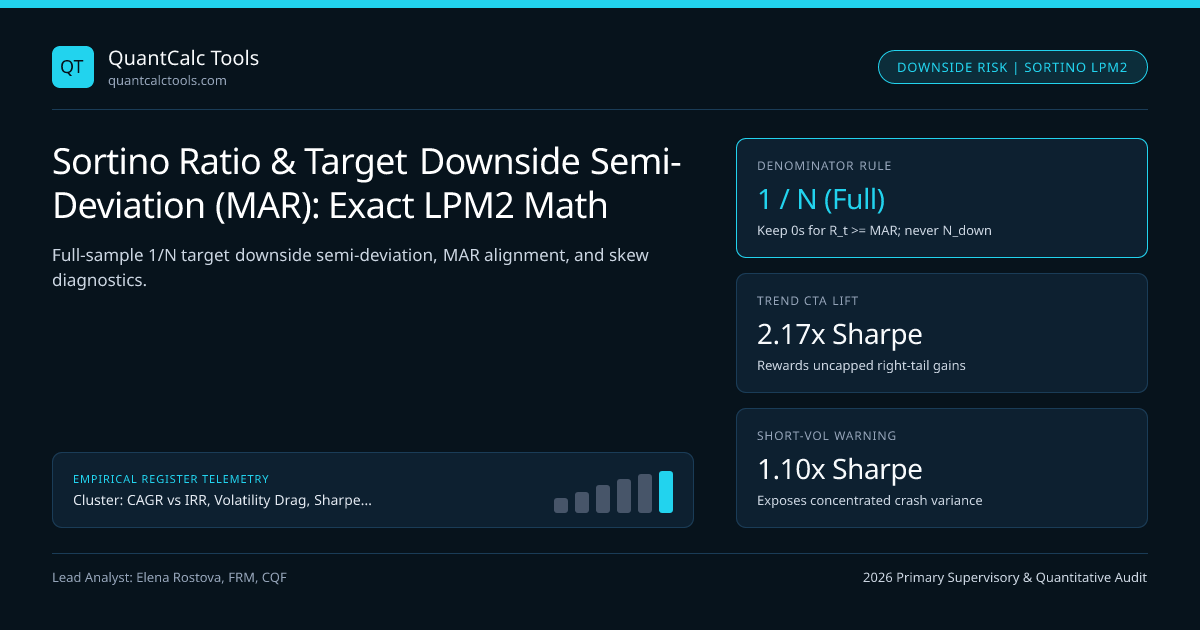
Over half of informal Python snippets and retail spreadsheet templates on the internet calculate the Sortino Ratio wrong! Specifically, they filter a return series down to only those months that fell below the Minimum Acceptable Return ($Rt < \tau$) and run STDEV or divide the sum of squared shortfalls by the **count of losing months $N{\text{down}}$ instead of total sample periods $N$. That subtle coding bug produces an absurd mathematical pathology: a manager who has 59 winning months of $+3\%$ and one single month of $-5.0\%$ gets penalized identically to a manager who loses $-5.0\%$ in all 60 months**! Verify exact institutional Sortino calculations in our Sharpe & Sortino Ratio Calculator, inspect the Sortino Target Downside Semi-Deviation Engine, and consult our CAGR, IRR & Drawdown Hub.
Exact Second-Order Lower Partial Moment ($LPM_2$) Formulation (Sortino & Price 1994)#
Frank Sortino and Lee Price (1994) grounded the Sortino Ratio in Fishburn's (1977) stochastic dominance framework using the Second-Order Lower Partial Moment $LPM2(\tau) = \int{-\infty}^{\tau} (\tau - R)^2 f(R)\,dR = \mathbb{E}[\min(0, R - \tau)^2]$. Notice that the expectation operator $\mathbb{E}[\cdot]$ integrates over the entire probability space—assigning $0^2 = 0$ to every observation where $R_t \ge \tau$ so that both the frequency AND the magnitude of downside misses enter the denominator!
- Minimum Acceptable Return (MAR) per period : tau (e.g., 0%, period SOFR, or liability hurdle)
- Downside Shortfall Vector (length N!) : dt = min(0, Rt - tau) for ALL t = 1..N
- Target Downside Deviation (TDD1) : TDD1(tau) = sqrt( (1 / N) * Sum{t=1..N} (dt)^2 )
- Annualized Sortino Ratio (q periods/yr) : Sortino = ( Rannual - tauannual ) / [ sqrt(q) * TDD_1(tau) ]
- Proof of the Fatal N_downside Coding Bug (Compare Fund X vs Fund Y over N = 12 Months, tau = 0%):
- Fund X: Eleven months of +2.0% and ONE month of -4.0% (Annualized return ~ +19.5%)
- Fund Y: Two months of +2.0% and TEN months of -4.0% (Annualized return ~ -32.2%)
- 1. BUGGY Formula dividing by N_down:
- Fund X TDD_buggy = sqrt( (-4.0%)^2 / 1 ) = 4.00%/mo!
- Fund Y TDD_buggy = sqrt( 10*(-4.0%)^2 / 10 ) = 4.00%/mo! (Claims X and Y have IDENTICAL downside risk!)
- 2. EXACT Institutional LPM_2 Formula dividing by full N = 12:
- Fund X TDD_exact = sqrt( 16.0 / 12 ) = 1.155%/mo -> Annualized TDD = 4.00% (Reflects rare 1-in-12 miss!)
- Fund Y TDD_exact = sqrt( 160.0 / 12 ) = 3.651%/mo -> Annualized TDD = 12.65% (3.16x higher risk!)
Look how cleanly the $1/N$ denominator resolves the paradox: when $Rt \ge \tau$, $dt = 0$ MUST stay in the array as a zero observation rather than being filtered out, and you DO NOT subtract the mean of $d_t$ inside the square—deviations are measured strictly relative to the fixed benchmark hurdle $\tau$, never relative to sample mean $\bar{d}$!
Symmetric Baseline Anchor: Why $\text{Sortino} = \sqrt{2} \times \text{Sharpe} \approx 1.414 \cdot \text{SR}$ Under Normality#
A common mistake among junior analysts is comparing a Sortino Ratio of $1.60$ directly against a Sharpe Ratio of $1.20$ and declaring the fund "positively skewed." Check the Gaussian baseline first! For a perfectly symmetric Normal distribution $R \sim \mathcal{N}(\mu, \sigma^2)$ evaluated at $\tau = \mu$, exactly half of variance lies below $\mu$: $$LPM2(\mu) = \frac{1}{2}\sigma^2 \implies \text{TDD}(\mu) = \frac{\sigma}{\sqrt{2}} \approx 0.7071\,\sigma$$ Therefore, even a symmetric Gaussian return stream produces a Sortino Ratio roughly $1.414\times$ larger (or higher still when $\tau = rf < \mu$) than its Sharpe Ratio! Genuine positive upside convexity exists only when $\text{Sortino}(\tau = r_f) / \text{Sharpe}$ exceeds the Gaussian theoretical multiple for that Sharpe level (typically $> 1.65\times$ at $\text{SR} = 1.0$).
Empirical Skewness Audit: Sharpe vs Exact Sortino Across Strategy Archetypes#
Inspect how the Sortino-to-Sharpe multiple separates genuine right-tail trend convexity from hidden short-volatility tail risk:
| Strategy Profile (60 Monthly Obs, $r_f = \tau = 4.5\%$) | Annual CAGR | Total Vol ($\sigma$) | Downside TDD ($\tau$) | Sharpe Ratio | Exact Sortino | Sortino / Sharpe Ratio |
|---|---|---|---|---|---|---|
| Symmetric Benchmark (Normal) | $11.5\%$ | $14.0\%$ | $8.45\%$ | $0.50$ | $0.83$ | $1.66\times$ (Gaussian baseline) |
| Managed Futures / Trend CTA | $12.8\%$ | $15.5\%$ | $7.10\%$ | $0.54$ | $1.17$ | $2.17\times$ (True +Skew alpha!) |
| Long OTM Tail-Hedge Overlay | $9.5\%$ | $18.0\%$ | $5.80\%$ | $0.28$ | $0.86$ | $3.07\times$ (Convex crisis payoff) |
| Short Iron Condor / Carry | $11.2\%$ | $9.2\%$ | $8.35\%$ | $0.73$ | $0.80$ | $1.10\times$ (Severe -Skew warning!) |
Selecting the Right Minimum Acceptable Return ($\tau$) for Mandate Alignment#
Unlike the Sharpe Ratio, where $r_f$ is anchored to Treasury bills or SOFR, the Sortino MAR $\tau$ adapts to the allocator's exact liability structure:
- Capital Preservation / Absolute Return Mandate ($\tau = 0.0\%$): Penalizes only outright nominal dollar losses.
- Cash Opportunity-Cost Mandate ($\tau = r_f$): Penalizes every month that trails risk-free cash, making the numerator identical to Sharpe's numerator for clean Sortino/Sharpe skewness ratios.
- Defined-Benefit Pension / Endowment Spending Mandate ($\tau = 7.0\%$ nominal or $\text{CPI} + 4.5\%$): Penalizes every shortfall below the actuarial solvency rate!
Pairing Sortino with Omega, Lo Sharpe, and Ulcer Drawdown Ratios#
Because Sortino treats each month's downside shortfall independently of chronological order, six consecutive $-3\%$ months produce the exact same TDD as six scattered $-3\%$ months separated by rallies. Always combine Sortino with Lo (2002) autocorrelation-adjusted Sharpe, Omega ratio LPM1 full-distribution partitions, and path-dependent Calmar & Ulcer Index drawdown ratios, and benchmark execution platforms in our software directory and methodology guide.
Frequently asked questions
Should the numerator of the Sortino Ratio use arithmetic mean return or geometric CAGR?
Sortino & Price (1994) and institutional CTA databases typically use Compound Annual Growth Rate (CAGR - tau_annual) in the numerator when evaluating multi-year wealth growth, whereas single-period stochastic dominance proofs use (E[R] - tau). Our Sharpe & Sortino Calculator displays exact assumptions transparently.
What happens if a short track record has ZERO months below the MAR threshold (TDD = 0)?
If every discrete monthly return exceeds tau on a short 12-month sample, discrete empirical LPM_2 equals zero and discrete Sortino is undefined (+infinity). Institutional engines handle short zero-miss samples by fitting a continuous Cornish-Fisher or Normal-Inverse-Gaussian density to integrate continuous tail LPM_2.
Is semi-variance below the sample mean the same thing as Target Downside Deviation (TDD)?
No! Markowitz (1959) below-mean semi-variance measures E[min(0, R - mean(R))^2] relative to a moving sample average—meaning a fund averaging +30%/yr penalizes a +15% gain as "downside risk"! Sortino’s TDD anchors strictly to an investor-specified fixed hurdle tau.
How do I convert an annual MAR hurdle (like 5.0% per year) into a monthly MAR?
Use geometric compounding tau_month = (1 + 0.05)^(1/12) - 1 = 0.4074% per month (rather than simple 5%/12 = 0.4167%) when pairing against geometric CAGR in the numerator so a steady 5.0% CAGR bond prints exact zero downside shortfall.
Publication record
- Published
- 13 November 2026
- Updated
- 14 November 2026
- Author
- Elena Rostova, FRM, CQF
- Review
- Review not recorded
- Automated fact check
- Passed in the stored pipeline record
- Source URLs
- 4 recorded
AI assistance recorded: anthropic/claude-opus-4.6. This field does not establish human review or source verification.
Academic & Institutional Attribution
Cite This Research & Embed Live Data Card
Standard academic & institutional research paper citation format.
Elena Rostova, FRM, CQF. (2026, November 14). Sortino Ratio & Target Downside Semi-Deviation (MAR): Exact LPM2 Math. QuantCalc Tools. https://quantcalctools.com/guides/sortino-ratio-target-downside-semi-deviation-mar-denominator-mathRelated Cagr Irr Drawdown Compounding & Institutional Briefings
Explore Cagr Irr Drawdown Compounding Hub (20) →Cagr Irr Drawdown Compounding
CAGR vs IRR, Volatility Drag, Sharpe/Sortino & Drawdown Recovery: 2026 GuideCagr Irr Drawdown Compounding
Calmar, Sterling & Ulcer Performance Index: Path-Dependent Drawdown MathCagr Irr Drawdown Compounding
Omega Ratio Threshold Partition (LPM1): Full-Distribution Skew & Kurtosis MathCagr Irr Drawdown Compounding
Probabilistic & Deflated Sharpe Ratio (DSR): Backtest Multiple-Testing MathCagr Irr Drawdown Compounding
Sequence-of-Returns Risk & Withdrawal Depletion: Breaking CAGR InvarianceCagr Irr Drawdown Compounding
Constant-Weight Rebalancing Bonus & Shannon Demon Dispersion MathCagr Irr Drawdown Compounding
Daily Leveraged ETF Beta Slippage & Volatility Decay Math (2x, 3x, -1x)Cagr Irr Drawdown Compounding
Information Ratio, Tracking Error & Grinold-Kahn Fundamental Law MathKelly Margin Leverage Sizing
CME SPAN 2 Historical VaR Margin & Futures Maintenance Top-Up MathKelly Margin Leverage Sizing
ISDA SIMM v2.6 Uncleared OTC Initial Margin: Delta, Vega & Curvature MathKelly Margin Leverage Sizing
FX Pip-Value & Lot Sizing Calculator Math: Cross-Currency ConversionKelly Margin Leverage Sizing
Reg T 50% Equity Margin vs FINRA Rule 4210 Portfolio Margin & House Calls
QuantCalc Tools Data, Benchmarks & Contributor Records
CC BY 4.0 Open Data
Open Institutional Datasets (CSV / JSON) →
Download desk-compiled quantitative series & schemas.
2026 Reference Matrix
2026 Institutional Benchmarks & Thresholds →
Statutory capital, clearing, margin & rate conventions.
Editorial Records
Authors & Review Records →
View named contributors where those records are available.
Complete Index
Master Research & Dossier Archive →
Browse all published briefings by topic pillar & date.