
Daily Leveraged ETF Beta Slippage & Volatility Decay Math (2x, 3x, -1x)
When an index finishes flat (+0.0%) over a volatile year with 32% annualized sigma, a 3x daily-reset ETF loses -26.5% before financing fees; master exact beta slippage and optimal leverage L*.
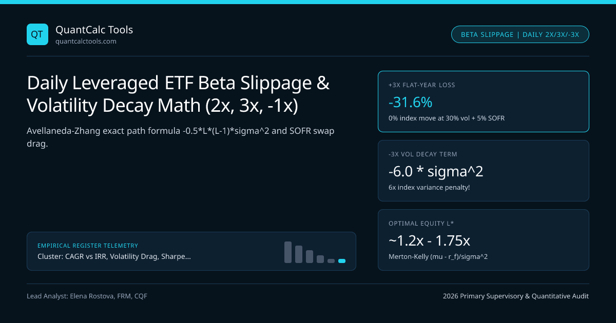
In volatile range-bound markets (such as 2022–2023 semiconductor or natural-gas swings, or 2008–2009 financials), retail investors routinely buy BOTH a +3x Bull Daily ETF and a -3x Bear Daily ETF on the same index, shocked six months later when both ETFs are down $-45\%$ simultaneously! Nothing is broken inside the ETF swap desk: daily-reset leveraged and inverse ETFs promise $L \times R_{\text{day}}$ over one single trading day, which forces the total-return swap desk to buy more exposure after every up day and sell exposure after every down day (pro-cyclical constant-leverage resetting—the exact opposite of Shannon's Demon contrarian rebalancing!). Model compounding drag in our CAGR Calculator, solve optimal $L^*$ in the Kelly Criterion Calculator, and explore our CAGR, IRR & Drawdown Hub.
Exact Continuous-Time Path Solution for Daily-Reset Leveraged ETFs (Avellaneda & Zhang 2010)#
Let underlying index $St$ follow $dSt / St = \mu\,dt + \sigma\,dWt$ with standalone geometric growth $gS = \mu - \frac{1}{2}\sigma^2$. A daily-reset ETF with leverage factor $L \in \mathbb{R}$ (e.g., $L = +2, +3, -1, -2, -3$), financing rate $rf$ (SOFR $+$ swap spread on $(L-1)$ borrowed notional), and expense ratio $f$ satisfies $dVt / Vt = [L\mu - (L-1)rf - f]\,dt + L\sigma\,dWt$. Integrating via Ito's Lemma expresses terminal ETF value $VT / V0$ directly as a function of terminal index ratio $(ST / S0)^L$ multiplied by an explicit exponential decay factor:
- VT / V0 = ( ST / S0 )^L * exp( [ -0.5 * L * (L - 1) * sigma^2 - (L - 1) * r_f - f ] * T )
- Equivalent Annualized Log-Growth Rate Comparing ETF (gETF) to Index (gS):
- gETF = L * gS - 0.5 * L * (L - 1) * sigma^2 - (L - 1) * r_f - f
- Verify Volatility Decay Term -0.5 * L * (L - 1) * sigma^2 Across Leverage Multipliers:
- L = +2x Bull : -0.5 * 2 * (1) * sigma^2 = -1.0 * sigma^2
- L = +3x Bull : -0.5 * 3 * (2) * sigma^2 = -3.0 * sigma^2 (3x variance multiplier on top of 3*g_S!)
- L = -1x Bear : -0.5 * (-1)(-2) sigma^2 = -1.0 * sigma^2! (-1x Inverse ETF STILL decays at -1.0*sigma^2!)
- L = -3x Bear : -0.5 * (-3)(-4) sigma^2 = -6.0 * sigma^2! (SIX TIMES index variance!)
- Worked 1-Year Flat-Index Audit (ST = S0 => +0.00% Net Index Change, sigma = 30.0%, r_f = 5.0%, f = 0.95%):
- 1. +3x Bull ETF : V1 / V0 = (1.00)^3 * exp( -3.0(0.09) - 2(0.05) - 0.0095 ) = exp(-0.3795) = 0.6842 (-31.58% Loss!)
- 2. -1x Bear ETF : V1 / V0 = (1.00)^(-1)exp( -1.0(0.09) - (-2)*(0.05) - 0.0095 ) = exp(+0.0005) ~= +0.05% (Short rebate offsets 30% vol!)
- 3. -3x Bear ETF : V1 / V0 = (1.00)^(-3)exp( -6.0(0.09) + 4*(0.05) - 0.0095 ) = exp(-0.3495) = 0.7050 (-29.50% Loss!)
Check those exact coefficients carefully—especially for inverse ETFs ($L < 0$), where textbook blogs often get the sign wrong! Because $L(L-1) = (-1)(-2) = +2 > 0$, a *-1x Inverse ETF suffers `-1.0 sigma^2 volatility decay** (identical to a +2x Bull ETF!), and a **-3x Inverse ETF suffers a staggering -6.0 * sigma^2` volatility decay*! Notice also the financing term $-(L-1)rf$: when $L = -1$, $-(L-1)rf = +2r_f$ (collateral cash interest plus short-swap rebate helps* inverse ETFs when SOFR is $5\%$, whereas $+3\times$ Bull ETFs pay $-2r_f = -10.0\%/\text{yr}$ in embedded swap financing!).
When Leveraged ETFs Outperform $L \times$ Cumulative Return: Strong Positive Momentum!#
Wait—how did TQQQ (+3x Nasdaq-100) surge over $+10{,}000\%$ during 2010–2021 despite -3.0 * sigma^2 volatility drag? Look back at the first factor in Avellaneda & Zhang's exact formula: $(ST / S0)^L$ is a power law ($x^3$), NOT linear $1 + 3(x - 1)$! In a smooth, low-volatility bull trend where the Nasdaq rises $+40\%$ (1.40x) with $\sigma = 16\%$ (-3 * 0.0256 = -7.68% vol decay) and low $1\%$ SOFR, $(1.40)^3 \times e^{-0.106} - 1 = 2.744 \times 0.899 - 1 =$ $+146.8\%$—crushing $3 \times 40\% = +120.0\%$ because daily resets compounded gains upward! Differentiating $g{\text{ETF}}(L)$ with respect to $L$ yields the exact Continuous Merton-Kelly Optimal Leverage: $$L^* = \frac{\mu - rf}{\sigma^2}$$ Whenever $L > 2L^*$, long-run Leveraged ETF CAGR drops below the unlevered $1\times$ index!
1-Year Leveraged & Inverse ETF Performance Matrix Across Volatility Regimes#
Compare exact realized compounding across flat, trending, and crashing markets for +2x, +3x, -1x, and -3x daily resets:
| ETF Leverage Tier ($r_f = 4.5\%$, $f = 0.90\%$) | Vol Decay Factor | Financing Drag | Flat Index ($0\%$, $\sigma=25\%$) | Bull Trend ($+25\%$, $\sigma=16\%$) | Choppy Crash ($-20\%$, $\sigma=38\%$) |
|---|---|---|---|---|---|
1x Unlevered Index | $0.0\,\sigma^2$ | $0.0\%$ | $0.0\%$ | $+25.0\%$ | $-20.0\%$ |
+2x Daily Bull ETF | $-1.0\,\sigma^2$ | $-4.5\%$ | $-11.1\%$ | $+43.4\%$ | $-48.5\%$ |
+3x Daily Bull ETF | $-3.0\,\sigma^2$ | $-9.0\%$ | $-24.9\%$ | $+61.9\%$ | $-74.2\%$ |
-1x Daily Inverse ETF | $-1.0\,\sigma^2$ | $+8.1\%$ (net) | $+1.8\%$ | $-21.5\%$ | $+16.4\%$ |
-3x Daily Inverse ETF | $-6.0\,\sigma^2$ | $+17.1\%$ (net) | $-19.2\%$ | $-55.6\%$ | $-1.9\%$ (Loses despite $-20\%$ crash!) |
Look at Row 5 of the Table: Why a -3x Bear ETF Can LOSE Money in a -20% Crash!#
Read the bottom-right cell of that table again: the underlying index crashed $-20.0\%$, yet the -3x Bear ETF ALSO lost $-1.9\%! Why? Because in a violent $-20\%$ bear market with $\sigma = 38\%$ annualized volatility (like 2008 financials or 2020 energy), $-6.0 \times 0.38^2 = -86.6\%$ of exponential volatility decay overwhelmed $(0.80)^{-3} = 1.953\times$ directional gain!
Risk Management & Regulatory Appropriateness Gates#
Both FINRA Regulatory Notice 09-31 and UK FCA / ESMA complex ETP rules classify daily leveraged ETPs as short-term tactical trading instruments rather than unmonitored buy-and-hold holdings. Compare static futures/margin leverage vs daily-reset ETFs using Half-Kelly continuous sizing, SOFR carry financing math, and arithmetic vs geometric variance drain.
Frequently asked questions
Why does a -1x Daily Inverse ETF have the exact same -1.0*sigma^2 volatility decay coefficient as a +2x Bull ETF?
Substitute L = -1 into -0.5 * L * (L - 1) * sigma^2: -0.5 * (-1) * (-2) * sigma^2 = -1.0 * sigma^2! Intuitively, when an index rises +10%, a -1x short ETF falls -10% (to $90) and must cover shorts to shrink notional; when the index drops back to 100 (-9.09%), the -1x ETF gains +9.09% on $90 = $98.18 (-1.82% round-trip loss).
Can you make risk-free money by shorting BOTH a +3x Bull ETF and a -3x Bear ETF to harvest volatility decay?
Institutional quant desks call this "shorting leveraged ETF pairs," and it is NOT risk-free! In a strong one-way directional trend (say +50% or -40% with low chop), the winning leg compounds exponentially via (S_T/S_0)^3 -> +237.5%, creating unlimited convex short-squeeze margin calls plus steep hard-to-borrow stock-loan fees.
What is the historically optimal constant leverage ratio L* for a broad US equity index like the S&P 500?
Using Merton-Kelly L* = (mu - r_f) / sigma^2 with long-run US equity excess arithmetic premium ~6.0% and annualized volatility ~18.5% (sigma^2 = 0.0342), full-Kelly L* ~= 1.75x—and institutional drawdown-constrained Half-Kelly sits near 0.9x to 1.25x, well below +3x!
Can a +3x Leveraged ETF go to zero in a single day?
In theory, a -33.34% single-day index drop wipes out 100% of a +3x ETF. On major US equity indices like the S&P 500, Level 3 market-wide circuit breakers halt trading for the remainder of the day at a -20.0% decline (-60% for a +3x S&P ETF), whereas un-halted commodity or single-stock 3x ETPs HAVE blown up intraday!
Publication record
- Published
- 13 November 2026
- Updated
- 14 November 2026
- Author
- Elena Rostova, FRM, CQF
- Review
- Review not recorded
- Automated fact check
- Passed in the stored pipeline record
- Source URLs
- 4 recorded
AI assistance recorded: anthropic/claude-opus-4.6. This field does not establish human review or source verification.
Academic & Institutional Attribution
Cite This Research & Embed Live Data Card
Standard academic & institutional research paper citation format.
Elena Rostova, FRM, CQF. (2026, November 14). Daily Leveraged ETF Beta Slippage & Volatility Decay Math (2x, 3x, -1x). QuantCalc Tools. https://quantcalctools.com/guides/daily-leveraged-etf-beta-slippage-volatility-decay-choppy-marketsRelated Cagr Irr Drawdown Compounding & Institutional Briefings
Explore Cagr Irr Drawdown Compounding Hub (20) →Cagr Irr Drawdown Compounding
CAGR vs IRR, Volatility Drag, Sharpe/Sortino & Drawdown Recovery: 2026 GuideCagr Irr Drawdown Compounding
Information Ratio, Tracking Error & Grinold-Kahn Fundamental Law MathCagr Irr Drawdown Compounding
Expected Maximum Drawdown of Brownian Motion (Magdon-Ismail Drift Math)Cagr Irr Drawdown Compounding
Simple vs Modified Dietz Return Formula: Sub-Period Cashflow Weighting MathCagr Irr Drawdown Compounding
Hedge Fund 2-and-20 Fee Drag, High-Water Mark & Hurdle Net CAGR MathCagr Irr Drawdown Compounding
Treynor Ratio, Jensen’s Alpha & Modigliani M-Squared (M2) Leverage MathCagr Irr Drawdown Compounding
Continuous Log Returns vs Simple Returns: Time Additivity vs Asset WeightsCagr Irr Drawdown Compounding
Fisher Exact Real CAGR, Inflation & Annual Tax Drag Compounding MathKelly Margin Leverage Sizing
Volatility-Target, Wilder ATR Stop-Loss & Equal Risk Contribution SizingKelly Margin Leverage Sizing
Central Clearing Variation Margin Liquidity Spirals & Cash Buffer MathKelly Margin Leverage Sizing
Ralph Vince Optimal f & Terminal Wealth Relative (TWR): Empirical Sizing MathKelly Margin Leverage Sizing
Short Naked Option Margin Math: Reg T 20%/10% Rule & Gamma Crash Expansion
QuantCalc Tools Data, Benchmarks & Contributor Records
CC BY 4.0 Open Data
Open Institutional Datasets (CSV / JSON) →
Download desk-compiled quantitative series & schemas.
2026 Reference Matrix
2026 Institutional Benchmarks & Thresholds →
Statutory capital, clearing, margin & rate conventions.
Editorial Records
Authors & Review Records →
View named contributors where those records are available.
Complete Index
Master Research & Dossier Archive →
Browse all published briefings by topic pillar & date.