
Continuous Log Returns vs Simple Returns: Time Additivity vs Asset Weights
Logarithmic returns are additive across time but NOT across portfolio assets; multiplying weights w_i by ln(P_t/P_{t-1}) misstates volatile multi-asset returns and breaks VaR/CAGR models.
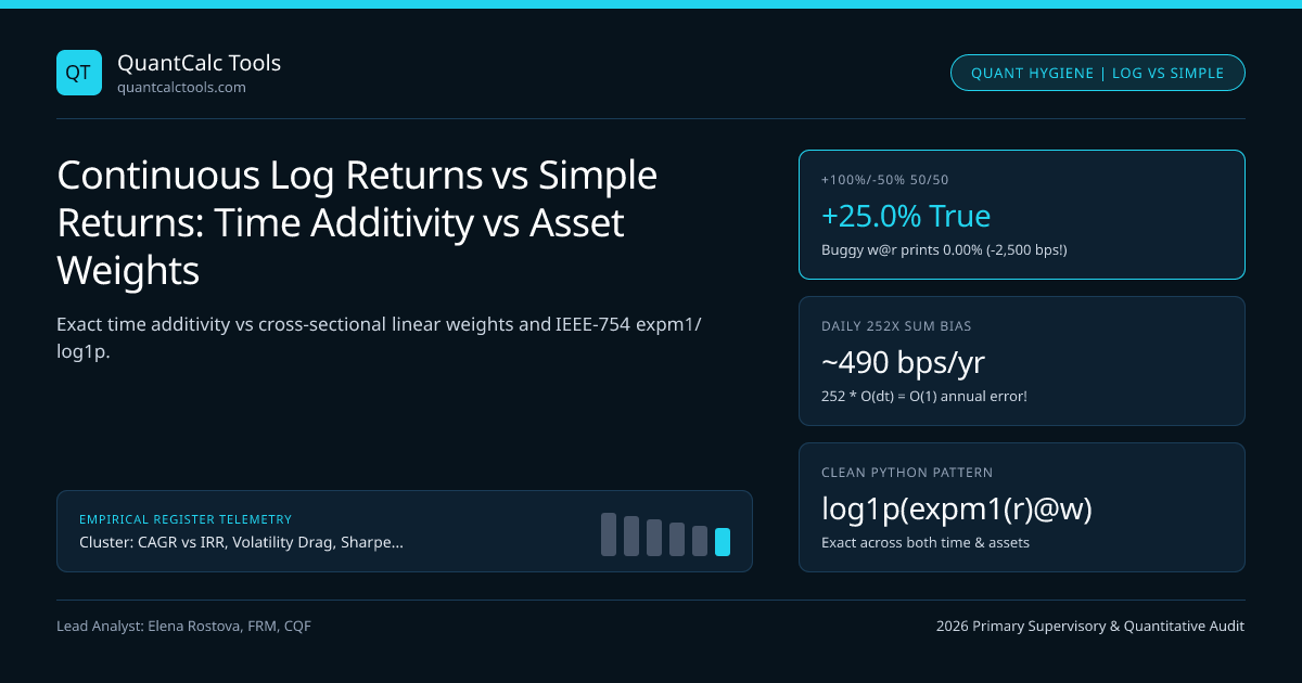
Reviewing junior quantitative research notebooks reveals one single bug more often than any other: computing daily asset log returns r = np.log(prices / prices.shift(1)), multiplying by portfolio weights r_port = (r @ weights), and summing r_port.cumsum! That one-liner violates conservation of dollars! Why? Because logarithmic returns add cleanly across time (t = 1..T), whereas simple linear returns add cleanly across portfolio constituents (i = 1..N)—and neither return convention is linear across both dimensions simultaneously! Audit exact compounding in our CAGR Calculator, inspect multi-asset risk in our Value-at-Risk Calculator, and consult the CAGR, IRR & Drawdown Hub.
Exact Identities & The Cross-Sectional Jensen Inequality Error#
Let $R{i,t} = (P{i,t} - P{i,t-1}) / P{i,t-1} \in (-1, \infty)$ be asset $i$'s simple discrete return and $r{i,t} = \ln(P{i,t} / P{i,t-1}) = \ln(1 + R{i,t}) \in (-\infty, \infty)$ be its continuously compounded log return ($R{i,t} = e^{r{i,t}} - 1$). Over $T$ time steps for a single asset, telescoping products turns $\ln(PT / P0)$ into an exact sum $\sum{t=1}^T rt$. Conversely, across $N$ assets held at beginning-of-period dollar weights $wi$ ($\sum wi = 1$ with $wi \ge 0$), dollar wealth linearity forces $R{p,t} = \sum{i=1}^N wi R_{i,t}$, meaning exact portfolio log return is the log of a weighted sum of exponentials:
- 1. Single-Asset Time Aggregation (Exact!) :
- r{1..T} = ln(PT / P0) = Sum{t=1..T} rt <=> CAGR = exp( (1/Tyrs) * Sum{t=1..T} rt ) - 1
- 2. Multi-Asset Portfolio Aggregation (Exact!):
- R{p,t} = Sum{i=1..N} (wi * R{i,t}) <=> r{p,t} = ln( Sum{i=1..N} [ wi * exp(r{i,t}) ] )
- 3. BUGGY Weighted Log-Return Formula & Exact Error Term (for w_i >= 0):
- rbuggy = Sum{i=1..N} (wi * r{i,t}) <= r_{p,t} [Strictly understates long-only returns by Jensen's Inequality!]
- Error = r{p,t} - Sum(wi * r{i,t}) ~= 0.5 * [ Sum(wi * r{i,t}^2) - (Sum wi * r_{i,t})^2 ] (Cross-sectional dispersion!)
- Worked Proof of the
weights @ log_returnsBug (50/50 Portfolio over 1 Period): - Asset 1 surges +100% (R1 = +1.00, r1 = ln(2.0) = +0.69315)
- Asset 2 crashes -50% (R2 = -0.50, r2 = ln(0.5) = -0.69315)
- True Dollar Wealth ($100 -> $50 in each): $50(2.0) + $50(0.5) = $100 + $25 = $125.00!
- > Exact Simple Return Rp = +25.00%; Exact Portfolio Log Return rp = ln(1.25) = +0.22314 (+22.31% log)!
- BUGGY
w @ rCode: 0.5(+0.69315) + 0.5(-0.69315) = 0.00000% (Claims portfolio made $0.00—off by -2,500 bps!)
Look at that result: weights @ log_returns told the researcher the portfolio made 0.00% ($100.00), when in reality the account balance sits at $125.00 (+25.00%)! And notice why the second-order error term $\frac{1}{2}[\sum wi ri^2 - (\sum wi ri)^2]$ looks so familiar: missing that cross-sectional dispersion term is literally throwing away the entire Booth-Fama / Shannon's Demon Rebalancing Bonus!
Even Worse on Short & Leveraged Portfolios: weights @ log_returns Hides Margin Wipeouts!#
For long-only weights ($wi \ge 0$), convexity of $e^x$ means w @ r systematically understates portfolio return. On **short or leveraged portfolios ($wi < 0$ or $\sum w_i > 1$), w @ r commits an infinitely more dangerous error in the opposite direction: suppose you short 100% of a meme stock ($w = -1.0$) that surges $+150\%$ overnight** ($R = +1.50$, $r = \ln(2.5) = +0.9163$).
- True Account Equity: $1 + (-1.0)(+1.50) = -0.50$ (
100%wiped out plus-50%negative-balance margin deficit!). - Buggy
w @ rCode: $\exp(-1.0 \times 0.9163) - 1 = e^{-0.9163} - 1 =$-60.0%loss—pretending $40\%$ of your equity survived a trade that bankrupted the account!
Domain Rules: Where to Use Log Returns, Simple Returns & Yield Differences#
Apply Attilio Meucci’s invariance separation across time-series simulation, Markowitz optimization, and fixed-income attribution:
| Quantitative Workflow Task | Use Log Returns ($rt = \ln(Pt/P_{t-1})$)? | Use Simple Returns ($Rt = Pt/P_{t-1}-1$)? | Mathematical Reason |
|---|---|---|---|
| Multi-Period Time Horizon Scaling | YES ($r{T} = \sum{t=1}^T r_t$) | No (products skew lognormally) | Central Limit Theorem & time additivity |
| GARCH / Cholesky Path Simulation | YES (for log-price assets) | Convert via $e^r - 1$ for PnL! | Guarantees simulated $PT = P0 e^{\sum r_t} > 0$ |
| Markowitz MVO / Portfolio Weights | No (breaks dollar additivity!) | YES ($\mu_p = w^\top \mathbb{E}[R]$) | Single-period wealth is linear in $R_i$ |
| Sharpe, Sortino & Brinson Attribution | No (distorts excess borrow $r_f$) | YES ($R{p,t} - r{f,t}$) | Margin financing & active weights are linear |
| Yield / Credit Spread Changes | NO! Use Differences $\Delta y_t$! | No ($y_t$ can cross $0\%$ / negative!) | Meucci "Quest for Invariance": rates add in bps |
Busting the Myth That "At Daily Frequency, Log and Simple Returns Are Identical!"#
Read the first metric box in the chart above very carefully—this shocks even experienced quants! On one single day, $|rt - Rt| \approx \frac{1}{2}Rt^2 \approx \frac{1}{2}\sigma{\text{daily}}^2$ really is tiny ($\sim 1.9\text{ bps}$ per day for $35\%$-vol stocks). When you sum $252$ daily errors across a year, $252 \times \frac{1}{2}\sigma{\text{daily}}^2 = \frac{1}{2}\sigma{\text{annual}}^2 =$ -612 bps per year! Higher sampling frequency does NOT make cumulative w @ r error vanish, because $N{\text{steps}} \times \mathcal{O}(1/N{\text{steps}}) = \mathcal{O}(1)$!
Applying Attilio Meucci's "Quest for Invariance" Across Asset Classes#
Follow Attilio Meucci's institutional architecture: model equity/FX spot invariants in log space (Cholesky Monte Carlo Engine), model interest rates and credit spreads in basis-point differences ($\Delta y_t$), map every instrument back to exact linear P&L at the horizon before applying weights or computing Cornish-Fisher VaR and arithmetic vs geometric variance drain, and verify production implementations in our methodology and proprietary software stack.
Frequently asked questions
Why doesn’t the difference between daily log returns and daily simple returns vanish over a 1-year backtest?
Because r_t = ln(1 + R_t) = R_t - 0.5*R_t^2 + O(R_t^3) differs from R_t by a SYSTEMATIC one-signed quadratic term (-0.5*R_t^2), not zero-mean noise! Summing -0.5*R_t^2 over 252 trading days accumulates quadratic variation -0.5*sigma_annual^2 regardless of how finely you slice Δt!
How do I convert an annualized log return mean (mu_log) into annualized CAGR?
Simply exponentiate and subtract one: CAGR = exp(mu_log) - 1! In fact, annualized sample mean log return (1 / T_years) * Sum_{t=1..N} r_t equals (1 / T_years) * ln(P_N / P_0), so exp(mean_annual_log_return) - 1 = (P_N / P_0)^(1 / T_years) - 1 === Exact Geometric CAGR!
Why shouldn’t I take log returns of bond yields or interest rates like ln(y_t / y_{t-1})?
Two reasons: first, sovereign yields (EUR, JPY, CHF in 2015–2022) and real TIPS yields frequently drop to 0% or turn negative, crashing ln(y_t); second, bond DV01 P&L scales linearly with basis-point yield CHANGES (y_t - y_{t-1}), not percentage yield ratios!
In numpy/pandas, what is the cleanest vectorized one-liner to compute exact rebalanced portfolio equity from log returns?
Given a (T x N) matrix log_ret and length-N weight vector w: write simple_port = (np.expm1(log_ret) @ w) and then equity_curve = np.exp(np.log1p(simple_port).cumsum) (using expm1 and log1p for full IEEE-754 floating-point precision on small returns!).
Publication record
- Published
- 13 November 2026
- Updated
- 14 November 2026
- Author
- Elena Rostova, FRM, CQF
- Review
- Review not recorded
- Automated fact check
- Passed in the stored pipeline record
- Source URLs
- 4 recorded
AI assistance recorded: anthropic/claude-opus-4.6. This field does not establish human review or source verification.
Academic & Institutional Attribution
Cite This Research & Embed Live Data Card
Standard academic & institutional research paper citation format.
Elena Rostova, FRM, CQF. (2026, November 14). Continuous Log Returns vs Simple Returns: Time Additivity vs Asset Weights. QuantCalc Tools. https://quantcalctools.com/guides/continuous-log-return-time-additivity-vs-simple-portfolio-weightsRelated Cagr Irr Drawdown Compounding & Institutional Briefings
Explore Cagr Irr Drawdown Compounding Hub (20) →Cagr Irr Drawdown Compounding
CAGR vs IRR, Volatility Drag, Sharpe/Sortino & Drawdown Recovery: 2026 GuideCagr Irr Drawdown Compounding
Fisher Exact Real CAGR, Inflation & Annual Tax Drag Compounding MathCagr Irr Drawdown Compounding
Arithmetic vs Geometric Mean Return: 0.5*Sigma^2 Variance Drain DerivationCagr Irr Drawdown Compounding
TWRR (CAGR) vs MWRR (XIRR): Irregular Cashflow Timing Divergence MathCagr Irr Drawdown Compounding
XIRR Newton-Raphson Convergence, Descartes Multiple Roots & MIRR MathCagr Irr Drawdown Compounding
Asymmetric Drawdown Recovery Hyperbola & Breakeven Compounding Time MathCagr Irr Drawdown Compounding
Sharpe Ratio IID Annualization Trap & Lo (2002) Autocorrelation HaircutCagr Irr Drawdown Compounding
Sortino Ratio & Target Downside Semi-Deviation (MAR): Exact LPM2 MathKelly Margin Leverage Sizing
Guaranteed Stop-Loss Order (GSLO) Premium vs Gap Slippage & Option MathMarket Insights
Cboe Global Markets (CBOE) Earnings Strength Keeps Valuation Debate In Focus - Yahoo FinanceRegulatory Compliance
Financial Stability Board to launch hedge fund leverage data consultation - Traders UnionMarket Insights
Rayonier jumped after earnings. Why we still see upside for the timber REIT
QuantCalc Tools Data, Benchmarks & Contributor Records
CC BY 4.0 Open Data
Open Institutional Datasets (CSV / JSON) →
Download desk-compiled quantitative series & schemas.
2026 Reference Matrix
2026 Institutional Benchmarks & Thresholds →
Statutory capital, clearing, margin & rate conventions.
Editorial Records
Authors & Review Records →
View named contributors where those records are available.
Complete Index
Master Research & Dossier Archive →
Browse all published briefings by topic pillar & date.