
Parametric Var Expected Shortfall
Filtered Historical Simulation (FHS): GARCH Bootstrap VaR & ES Math Guide
Barone-Adesi Filtered Historical Simulation (FHS) marries GARCH conditional volatility responsiveness with non-parametric empirical fat tails and cross-asset rank dependence.
Unfiltered Historical Simulation (HS) preserves empirical fat tails and non-linear asset co-movements without imposing Gaussian formulas, yet fails Christoffersen Markov independence backtests whenever market volatility shifts regimes: feeding a calm 2025 return window into an autumn volatility spike understates 1-day VaR by half, whereas feeding crisis returns into a quiet market overcharges capital for twelve months. Pioneered by Barone-Adesi, Giannopoulos, and Vosper (1999), Filtered Historical Simulation (FHS) eliminates that trade-off—and today powers clearinghouse margin engines including LCH ForexClear and components of CME SPAN 2 Historical & Stress VaR. Benchmark parametric normal outputs in our Value at Risk (VaR) calculator and review our Parametric VaR & Expected Shortfall calibration guide.
De-Volatilization and Re-Volatilization: Exact FHS Equations#
Suppose we observe $T = 500$ historical daily returns $r1, \dots, rT$ and fit an asymmetric GJR-GARCH(1,1) conditional mean and variance path $(\hat{\mu}t, \hat{\sigma}t)$ for each day $t = 1, \dots, T$, plus tomorrow's conditional forecast $(\hat{\mu}{T+1}, \hat{\sigma}{T+1})$:
- Extract Standardized Empirical Innovations ($\hat{z}_t$):
$$\hat{z}t = \frac{rt - \hat{\mu}t}{\hat{\sigma}t}, \qquad t = 1, \dots, T$$ Dividing each historical return by the conditional volatility prevailing on that historical date strips out volatility clustering, transforming raw returns into approximately i.i.d. draws that retain true empirical skewness, kurtosis, and cross-asset crash co-dependence!
- Re-Scale to Tomorrow's Volatility State ($\tilde{r}_{T+1}^{(t)}$):
$$\tilde{r}{T+1}^{(t)} = \hat{\mu}{T+1} + \hat{\sigma}{T+1} \cdot \hat{z}t, \qquad t = 1, \dots, T$$
Worked Barone-Adesi GARCH De-Volatilization & Re-Scaling Audit#
- Historical Window: T = 500 Trading Days; Target Metric: 97.5% Expected Shortfall (Worst 2.5% = Top 12.5 Losses)
- Current Market State: Post-BoE Surprise Volatility Spike -> Tomorrow's GARCH Forecast sigma_{T+1} = 1.65%
- Historical Worst Tail Days (Raw Loss vs Prevailing Historical GARCH Volatility sigma_t):
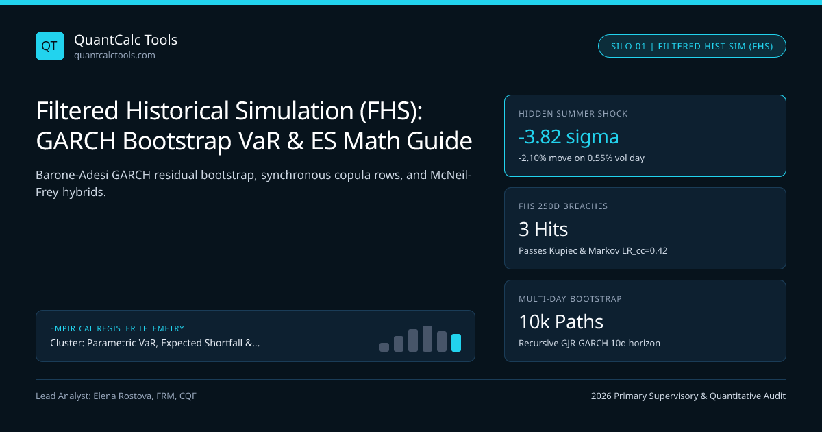
- Obs #114 (Quiet Summer Flash Dip): r114 = -2.10%, Prevailing sigma114 = 0.55% => z_114 = -3.8182!
- Obs #302 (Prior Crisis Selloff): r302 = -3.60%, Prevailing sigma302 = 1.80% => z_302 = -2.0000!
- 1) Unfiltered Historical Simulation Distortion:
- Ranks Obs #302 (-3.60% = -$1,440,000) as far worse than Obs #114 (-2.10% = -$840,000),
- ignoring that tomorrow's vol (1.65%) is 3x higher than Day 114's vol!
- Unfiltered 97.5% ES across raw 500-day average vol (0.88%) = $896,000.
- 2) Filtered Historical Simulation Re-Scaling at sigma_{T+1} = 1.65%:
- Re-scaled Obs #114 = 1.65% * (-3.8182) = -6.3000% (-$2,520,000!)
- Re-scaled Obs #302 = 1.65% * (-2.0000) = -3.3000% (-$1,320,000 — drops out of worst 2.5% tail!)
- Average of Worst 12.5 Standardized Residuals E[-z | z <= q_0.025] = 2.7420
- FHS 1-Day 97.5% ES = $40,000,000 * 0.0165 * 2.7420 = $1,809,720 (+101.98% timely risk capture!)
Examine that reversal between Observation #114 and Observation #302! A raw $-2.10\%$ drop occurring during a sleepy $0.55\%$-volatility summer was actually a $-3.82\sigma$ structural shock; scaling that innovation to today's $1.65\%$ conditional volatility reveals a latent $-6.30\%$ crash scenario that raw Historical Simulation completely buries!
Multi-Day Recursive Path Bootstrapping & Synchronous Cross-Asset Vectors#
How do you extend FHS from a 1-day risk horizon to a 10-day Basel III FRTB 97.5% Expected Shortfall horizon without invoking $\sqrt{10}$? You cannot just sort 1-day residuals! Instead, run $B = 10,000$ recursive path simulations of length $H = 10$ days:
- On step $k = 1, \dots, 10$ of path $b$, draw a single random historical date index $d^* \in \{1, \dots, T\}$ uniformly with replacement.
- Apply the entire cross-sectional row vector $(\hat{z}{d^*, 1}, \hat{z}{d^, 2}, \dots, \hat{z}_{d^, N})$ simultaneously across all $N$ assets! Drawing the same historical date $d^*$ across every asset automatically preserves non-Gaussian empirical tail dependence (copula crash synchronization) without inverting a $N \times N$ correlation matrix!
- Compute each asset's Day $T+k$ simulated return $r{T+k, i}^{(b)} = \hat{\mu}{T+k, i} + \hat{\sigma}{T+k, i}^{(b)}\hat{z}{d^*, i}$, feed $(r{T+k, i}^{(b)})^2$ directly into asset $i$'s GJR-GARCH equation to obtain $\hat{\sigma}{T+k+1, i}^{(b)}$ for the next step, and compound the 10-day path!
Unfiltered Historical Simulation vs Parametric GARCH vs FHS Comparison#
| Simulation / VaR Paradigm | Volatility Responsiveness | Tail Distribution Shape | Multi-Asset Crash Copula | Procyclicality Floor Needed? |
|---|---|---|---|---|
| Unfiltered Historical Simulation | Very Slow (Ghost effects) | Empirical (Capped at max loss) | Exact historical dates | Low (Sticky crisis memory) |
| Gaussian Parametric / EWMA | Fast (EWMA vs GARCH) | Thin mesokurtic ($K_e=0$) | Linear Pearson $\Sigma$ only | High (Needs vol floor) |
| Filtered Historical Simulation (FHS) | Fast (GJR-GARCH scaled) | Empirical standardized $z_t$ | Exact synchronous row copula | Moderate (EMIR 25% floor) |
| FHS + EVT GPD Hybrid (McNeil-Frey) | Fast (GJR-GARCH scaled) | Smooth Pareto extrapolation | Empirical + GPD marginals | Best-in-class extreme tail |
| Cholesky Normal Monte Carlo | Model-dependent | Parametric only | Elliptical MONTE-CARLO-CHOLESKY | Model-dependent |
Eliminating Sample Ceiling Bias via McNeil-Frey FHS-EVT#
Standard FHS has one remaining limitation at ultra-high confidence levels (such as 99.9% CCP default-fund stress): a 500-day residual pool contains zero observations beyond $\mint(\hat{z}t)$. McNeil & Frey (2000) solved this permanently by fitting a Generalized Pareto Distribution (GPD) to standardized GARCH residuals exceeding the 90th or 95th loss percentile—see our companion derivation in Extreme Value Theory Peaks-Over-Threshold GPD tail ES. Audit broker margin methodologies across venues like BP Prime and explore all 20 guides on the Parametric VaR & Expected Shortfall Topic Hub.
Frequently asked questions
Why must standardized GARCH residuals be re-centered and variance-normalized before running FHS?
In finite samples of 500 days, quasi-maximum-likelihood GARCH residuals often exhibit a sample mean slightly off zero and sample standard deviation around 0.98 or 1.02; enforcing exact zero mean and unit variance prevents compounding bias across 10-day bootstrap horizons.
How does Filtered Historical Simulation handle correlations across 200 portfolio assets?
Instead of estimating 19,900 pairwise correlations, FHS fits 200 univariate GJR-GARCH filters and bootstraps historical calendar dates synchronously across all 200 residual columns, preserving exact historical rank correlation and joint tail jumps.
What happens if a newly listed stock or bond has fewer than 500 historical days in an FHS engine?
Missing pre-IPO history breaks synchronous date-row sampling unless backfilled via factor-model regression against sector/curve benchmarks plus idiosyncratic residual draws, as permitted under Basel MAR33 proxy-data rules.
Why do central counterparties add a 25% anti-procyclicality floor to FHS initial margin?
During prolonged tranquil markets, GARCH volatility drops toward historic lows, shrinking FHS margin and encouraging excess leverage. EMIR RTS rules require CCPs to floor FHS volatility or blend a 25% buffer calibrated to stressed periods.
Publication record
- Published
- 14 November 2026
- Updated
- 14 November 2026
- Author
- Elena Rostova, FRM, CQF
- Review
- Review not recorded
- Automated fact check
- Passed in the stored pipeline record
- Source URLs
- 3 recorded
AI assistance recorded: anthropic/claude-opus-4.6. This field does not establish human review or source verification.
Academic & Institutional Attribution
Cite This Research & Embed Live Data Card
Standard academic & institutional research paper citation format.
Elena Rostova, FRM, CQF. (2026, November 14). Filtered Historical Simulation (FHS): GARCH Bootstrap VaR & ES Math Guide. QuantCalc Tools. https://quantcalctools.com/guides/filtered-historical-simulation-garch-standardized-residual-varRelated Parametric Var Expected Shortfall & Institutional Briefings
Explore Parametric Var Expected Shortfall Hub (20) →Parametric Var Expected Shortfall
Parametric VaR, Expected Shortfall & Fat-Tail Risk Calibration: 2026 Quantitative GuideParametric Var Expected Shortfall
Extreme Value Theory (EVT) Peaks-Over-Threshold: GPD VaR & ES Formula GuideParametric Var Expected Shortfall
Cholesky Factorization in Monte Carlo VaR: Fixing Broken Correlation GridsParametric Var Expected Shortfall
FRTB Stressed Expected Shortfall: Reduced-Factor MAR33.5 Calibration MathParametric Var Expected Shortfall
Acerbi-Szekely Expected Shortfall Backtesting: Non-Elicitability & Z2 MathParametric Var Expected Shortfall
Ledoit-Wolf Covariance Shrinkage in Portfolio VaR: Eigenvalue ConditioningParametric Var Expected Shortfall
Correlation Breakdown in Multi-Asset VaR: Stressed-Beta Contagion MathParametric Var Expected Shortfall
Garman-Klass & Yang-Zhang OHLC Volatility: Efficient VaR Input Math GuideBond Duration Convexity Math
Zero-Coupon STRIPS Convexity Scaling: Quadratic Maturity Leverage MathBond Duration Convexity Math
Par Swap DV01 vs Zero-Rate PV01: Jacobian Curve Transformation MathBond Duration Convexity Math
ACT/ACT ICMA vs 30/360 Accrued Interest & Odd-Stub Duration Bias MathBond Duration Convexity Math
TIPS Real-Yield Duration vs Nominal Treasury Empirical Beta Hedging Math
QuantCalc Tools Data, Benchmarks & Contributor Records
CC BY 4.0 Open Data
Open Institutional Datasets (CSV / JSON) →
Download desk-compiled quantitative series & schemas.
2026 Reference Matrix
2026 Institutional Benchmarks & Thresholds →
Statutory capital, clearing, margin & rate conventions.
Editorial Records
Authors & Review Records →
View named contributors where those records are available.
Complete Index
Master Research & Dossier Archive →
Browse all published briefings by topic pillar & date.