
Parametric Var Expected Shortfall
Acerbi-Szekely Expected Shortfall Backtesting: Non-Elicitability & Z2 Math
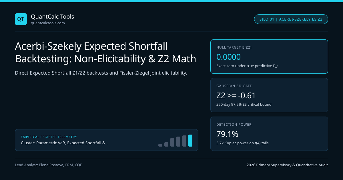
Gneiting proved standalone Expected Shortfall lacks a strictly consistent scoring function, yet Acerbi and Szekely’s unconditional Z2 statistic directly backtests joint VaR-ES tail severity without nuisance parameters.
When Gneiting (2011) proved mathematically that Expected Shortfall is not standalone elicitable—meaning no strictly consistent loss function exists whose minimization uniquely recovers true $ES\alpha$—critics initially claimed Basel III FRTB 97.5% Expected Shortfall could never be backtested! Acerbi & Székely (2014) and Fissler & Ziegel (2016) overturned that misconception completely: **backtesting (hypothesis testing against $H0$) is distinct from elicitability (point forecast ranking), and furthermore the joint pair $(VaR\alpha, ES\alpha)$ IS strictly jointly elicitable!** Compute baseline normal VaR and ES pairs in our Value at Risk (VaR) calculator and review our Parametric VaR & Expected Shortfall calibration guide.
Exact Acerbi-Székely $Z1$ and $Z2$ Backtesting Equations#
Let $Xt$ denote portfolio PnL on day $t \in \{1, \dots, T\}$ (negative values are losses), while $VaR{t,\alpha} > 0$ and $ES{t,\alpha} > 0$ denote positive loss forecasts at tail probability $p = 1 - \alpha = 0.025$ (for 97.5% ES), with breach indicator $It = \mathbb{I}{\{Xt + VaR{t,\alpha} < 0\}}$. Under a correctly specified conditional return distribution $H0$:
- Conditional Tail Severity ($Z_1$): Tests solely whether realized losses on breach days average $ES{t,\alpha}$, conditioning on $NT = \sum{t=1}^T It > 0$:
$$Z1 = \frac{1}{NT}\sum{t=1}^T \frac{Xt \cdot It}{ES{t,\alpha}} + 1, \qquad \mathbb{E}{H0}[Z1 \mid NT > 0] = 0$$
- Unconditional Joint Tail Test ($Z_2$): Replaces random $N_T$ in the denominator with expected hits $T \cdot (1 - \alpha)$, simultaneously testing breach frequency AND breach magnitude in one unified statistic:
$$Z2 = \frac{1}{T(1 - \alpha)}\sum{t=1}^T \frac{Xt \cdot It}{ES{t,\alpha}} + 1, \qquad \mathbb{E}{H0}[Z2] = 0$$
Worked Non-Parametric Acerbi-Szekely Z2 Test Statistic Audit#
- Observed Breaches over 250 Days: N_T = 7 Breach Days (Passes Kupiec 97.5% window [2, 12]!)
- Normalized Breach Ratios (-Xt / ES{t,0.975} on the 7 breach days, where X_t < 0):
- Day 19: -$3.40M / $2.50M = 1.360 Day 142: -$4.20M / $2.60M = 1.615
- Day 54: -$2.95M / $2.40M = 1.229 Day 188: -$3.85M / $2.50M = 1.540
- Day 91: -$3.10M / $2.50M = 1.240 Day 219: -$4.55M / $2.60M = 1.750
- Day 112:-$3.60M / $2.55M = 1.412
- Sum of Signed Ratios Sum(Xt * It / ES_t) = -(1.360 + 1.229 + 1.240 + 1.412 + 1.615 + 1.540 + 1.750) = -10.146
- 1) Conditional Severity Statistic Z_1:
- Z_1 = (-10.146 / 7) + 1 = -1.4494 + 1 = -0.4494 (< -0.26 critical -> TAIL SEVERITY UNDERSTATED!)
- 2) Unconditional Joint Statistic Z_2 (Divides by Expected Hits T*(1-alpha) = 6.25):
- Z_2 = (-10.146 / 6.25) + 1 = -1.6234 + 1 = -0.6234 (<< -0.70 5% normal critical? Close to 1% reject!)
- Note: Under Student-t(5) Monte Carlo null at T=250, 5% critical value for Z_2 is approx -0.72;
- under Gaussian null at T=250, 5% left-tail critical value for Z_2 is -0.608 -> REJECTS GAUSSIAN ES!
Look at what happened on those 7 breach days: Kupiec's 97.5% VaR frequency test passed effortlessly ($NT = 7$ vs $6.25$ expected, well below the 12-hit cutoff in Kupiec POF likelihood-ratio zones)! Yet on every single breach day, realized losses exceeded $ES{t,0.975}$ by $23\%$ to $75\%$, driving $Z1 = -0.4494$ and $Z2 = -0.6234$ deep into left-tail rejection territory! Sign convention reminder: negative $Z1$ or $Z2$ signals risk underestimation; positive values near $+1.0$ signal conservative over-margining.
Fissler-Ziegel (2016) Jointly Elicitable Scoring Function ($FZ_0$)#
What if a quantitative research team wants to rank two competing forecasting models—say, Student-t Expected Shortfall versus EVT Peaks-Over-Threshold GPD—on out-of-sample data without knowing the "true" data-generating distribution? Fissler, Ziegel & Gneiting (2016) derived the 0-homogeneous strictly consistent joint loss function (writing $v < 0$ for negative PnL quantile and $e \le v < 0$ for negative PnL ES): $$S{FZ0}(v, e, x) = -\frac{1}{e}\left(e - v + \frac{(v - x)\,\mathbb{I}{\{x \le v\}}}{1 - \alpha}\right) + \ln(-e) - 1$$ Minimizing average $S{FZ0}$ across out-of-sample days is mathematically guaranteed (via Diebold-Mariano tests) to select the model closest to the true conditional $(VaR\alpha, ES_\alpha)$ pair!
Comparing Expected Shortfall Backtesting & Elicitability Frameworks#
| ES Backtest Method | Requires Full Distribution $F_t$? | Tests Frequency + Magnitude? | Small-Sample Critical Values | Primary Institutional Strength |
|---|---|---|---|---|
| Basel MAR32 Dual-VaR Proxy | No (97.5% & 99% quantiles) | Indirectly via 2 quantiles | Exact Binomial | Simple statutory desk gate |
| McNeil-Frey Excess Residual Bootstrap | No (Tail residuals only) | Conditional Magnitude only | Non-parametric bootstrap | Isolates pure GPD tail shape error |
| Acerbi-Székely $Z_1$ Test | Yes (For null MC criticals) | Conditional Magnitude only | Insensitive to fat-tail null! | Immune to VaR frequency error |
| Acerbi-Székely $Z_2$ Test | Yes (Simulated predictive $F_t$) | Yes (Joint VaR + ES) | Stable (~$-0.61$ to $-0.74$) | High power against both errors |
| Fissler-Ziegel $S_{FZ0}$ Diebold-Mariano | No (Point $vt, et$ only!) | Yes (Comparative ranking) | Asymptotic HAC t-stat | Ranks rival engines without $H_0$ |
Ridge Backtesting & Berkowitz PIT Tail Censored Likelihood#
In addition to $Z2$, Acerbi & Székely (2017) introduced Ridge Backtesting based on Fissler-Ziegel's elicitability ridge, while Du & Escanciano (2017) generalized Christoffersen's autocorrelation test to cumulative Probability Integral Transforms (PIT) $ut = Ft(Xt)$ inside the 2.5% tail. Combine $Z_2$ validation with Christoffersen Markov independence testing, benchmark against the FRTB-ES-975 2026 Standard under UK PRA model validation guidance, and explore the Parametric VaR & Expected Shortfall Topic Hub.
Frequently asked questions
Does non-elicitability mean Expected Shortfall cannot be backtested?
No. Elicitability concerns whether a standalone point forecast minimizes an expected scoring rule for relative model ranking. Hypothesis testing (backtesting) evaluates whether realized tail losses match a model’s predicted distribution, which Acerbi-Szekely Z2 solves cleanly.
Why does Acerbi-Szekely Z2 outperform Z1 when VaR itself is miscalibrated?
Both Z1 and Z2 divide X_t by ES_t on days breaching VaR_t. However, Z1 divides by actual breaches N_T (which can mask parallel underestimation of both VaR and ES), whereas Z2 divides by expected breaches T*(1 - alpha), penalizing excess hit counts and severe losses together.
How do you obtain exact critical values for the Acerbi-Szekely Z2 test over 250 days?
Simulate M = 10,000 independent 250-day paths from the model’s own predictive return distribution F_t, compute Z2 on each path, and read the 5th and 1st empirical percentiles (typically around -0.61 and -0.92 under normality at 97.5% ES).
How does Fissler-Ziegel FZ0 scoring avoid unit-scale distortion across volatile and calm eras?
Because FZ0 is strictly 0-homogeneous—dividing forecast errors by negative ES and adding ln(-e)—high-volatility crisis weeks do not dominate the multi-year average score purely due to dollar scale, unlike quadratic scoring functions.
Publication record
- Published
- 14 November 2026
- Updated
- 14 November 2026
- Author
- Elena Rostova, FRM, CQF
- Review
- Review not recorded
- Automated fact check
- Passed in the stored pipeline record
- Source URLs
- 3 recorded
AI assistance recorded: anthropic/claude-opus-4.6. This field does not establish human review or source verification.
Academic & Institutional Attribution
Cite This Research & Embed Live Data Card
Standard academic & institutional research paper citation format.
Elena Rostova, FRM, CQF. (2026, November 14). Acerbi-Szekely Expected Shortfall Backtesting: Non-Elicitability & Z2 Math. QuantCalc Tools. https://quantcalctools.com/guides/acerbi-szekely-expected-shortfall-backtesting-z2-statisticRelated Parametric Var Expected Shortfall & Institutional Briefings
Explore Parametric Var Expected Shortfall Hub (20) →Parametric Var Expected Shortfall
Parametric VaR, Expected Shortfall & Fat-Tail Risk Calibration: 2026 Quantitative GuideParametric Var Expected Shortfall
Ledoit-Wolf Covariance Shrinkage in Portfolio VaR: Eigenvalue ConditioningParametric Var Expected Shortfall
Correlation Breakdown in Multi-Asset VaR: Stressed-Beta Contagion MathParametric Var Expected Shortfall
Garman-Klass & Yang-Zhang OHLC Volatility: Efficient VaR Input Math GuideParametric Var Expected Shortfall
Lognormal vs Arithmetic Parametric VaR: Multi-Month Horizon Math GuideParametric Var Expected Shortfall
Basel FRTB Non-Modellable Risk Factors (NMRF): RFET & SES Capital MathParametric Var Expected Shortfall
Cornish-Fisher VaR Quantile Expansion: Skewness & Excess Kurtosis Formula GuideParametric Var Expected Shortfall
Student-t Expected Shortfall Formula: Degrees-of-Freedom & Unit-Variance ScalingBond Duration Convexity Math
Spread Duration vs Duration-Times-Spread (DTS): Credit Hedging MathBond Duration Convexity Math
Floating-Rate Note (FRN) Interest-Rate Reset Duration vs Spread Duration MathBond Duration Convexity Math
Ultra-Long 50Y Gilt & 100Y Century Bond Convexity Asymmetry MathBond Duration Convexity Math
Principal Component Analysis (PCA) Level, Slope & Curvature DV01 Hedging Math
QuantCalc Tools Data, Benchmarks & Contributor Records
CC BY 4.0 Open Data
Open Institutional Datasets (CSV / JSON) →
Download desk-compiled quantitative series & schemas.
2026 Reference Matrix
2026 Institutional Benchmarks & Thresholds →
Statutory capital, clearing, margin & rate conventions.
Editorial Records
Authors & Review Records →
View named contributors where those records are available.
Complete Index
Master Research & Dossier Archive →
Browse all published briefings by topic pillar & date.