
Parametric Var Expected Shortfall
Lognormal vs Arithmetic Parametric VaR: Multi-Month Horizon Math Guide
Linear arithmetic VaR reports absurd 116% losses on unlevered 50%-volatility positions over 1-year horizons; exact lognormal transformation bounds losses below 100% while accounting for Ito drift.
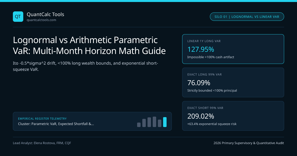
Plug an unlevered $$10,000,000$ long position in a $55\%$-annual-volatility biotechnology or digital-asset basket into a naive 1-year linear arithmetic 99% VaR formula ($VaR = W \cdot z{0.99} \cdot \sigmaa$), and the spreadsheet outputs $VaR_{99} = \$10\text{M} \times 2.32635 \times 0.55 = \$12,794,925$—a 127.95% loss on an unlevered cash asset that cannot legally drop below $$0$! That embarrassing mathematical impossibility arises whenever risk analysts conflate continuously compounded log returns $r{log} = \ln(ST / S0)$ with discrete percentage wealth changes $R{simple} = (ST - S0)/S0 = e^{r{log}} - 1$. Compare 1-day linear approximations in our Value at Risk (VaR) calculator, inspect long-horizon compounding in our CAGR calculator, and review our Parametric VaR & Expected Shortfall calibration guide.
Exact Geometric Brownian Motion Lognormal VaR & Expected Shortfall#
Suppose asset price $St$ follows Geometric Brownian Motion $dSt / St = \mu\,dt + \sigma\,dWt$, where $\mu$ is annualized arithmetic drift and $\sigma$ is annualized log-return volatility. By Itô's Lemma, terminal log return over horizon $T$ (in years) is normally distributed with variance-drained geometric mean $(\mu - \frac{1}{2}\sigma^2)T$: $$\ln\!\left(\frac{ST}{S0}\right) \sim \mathcal{N}\!\Big(\big(\mu - \tfrac{1}{2}\sigma^2\big)T,\;\; \sigma^2 T\Big)$$ Exponentiating the left-tail quantile $q{log} = (\mu - \frac{1}{2}\sigma^2)T - z\alpha\sigma\sqrt{T}$ yields Exact Lognormal Relative VaR (strictly bounded inside $[0, W)$ for all $\sigma, T < \infty$), and integrating the lognormal lower tail yields Exact Closed-Form Lognormal Expected Shortfall:
$$VaR{\alpha}^{log} = W\left[1 - \exp\!\Big(\big(\mu - \tfrac{1}{2}\sigma^2\big)T - z\alpha \sigma\sqrt{T}\Big)\right]$$
$$ES{\alpha}^{log} = W\left[1 - \frac{e^{\mu T}}{1 - \alpha}\,\Phi\!\left(-z\alpha - \sigma\sqrt{T}\right)\right]$$
Worked 1-Year Distressed-Vol VaR Audit: Linear >100% Bug vs Exact Lognormal#
- Inputs: W = $10,000,000, Horizon T = 1.00 Year, Annualized Volatility sigma = 55.0% (0.55)
- Arithmetic Expected Return mu = +12.0% => Geometric Log Drift = 0.12 - 0.5*(0.55)^2 = -0.03125 (-3.125%!)
- 1) Naive Linear Arithmetic 99% VaR (Broken Formula: W * (z_0.99 * sigma - mu)):
- VaR_99(linear) = $10,000,000 * (2.32635 * 0.55 - 0.12) = $11,594,925 (115.95% LOSS — IMPOSSIBLE!)
- Zero-Mean Linear 99% VaR = $12,794,925 (127.95% LOSS — IMPOSSIBLE!)
- 2) Exact Lognormal 99.0% VaR (z_0.99 = 2.32635):
- Log Quantile q_0.01 = -0.03125 - 2.32635 * 0.55 = -0.03125 - 1.27949 = -1.31074
- Terminal Wealth Ratio ST / S0 = exp(-1.31074) = 0.26962 (Asset falls to 26.96 cents on the dollar)
- Exact Lognormal VaR_99 = $10,000,000 * (1 - 0.26962) = $7,303,799 (73.04% Loss — Physically Valid!)
- 3) Exact Lognormal 97.5% Expected Shortfall (z_0.975 = 1.95996, 1 - alpha = 0.025):
- Shifted Normal Argument = -1.95996 - 0.55 = -2.50996 => Phi(-2.50996) = 0.0060373
- ES_97.5(lognormal) = $10,000,000 * [ 1 - (exp(0.12) / 0.025) * 0.0060373 ]
- = $10,000,000 * [ 1 - 45.0999 * 0.0060373 ] = $7,277,185 (72.77% Tail Mean Loss!)
Look at the beauty of that closed-form Lognormal ES equation $W[1 - \frac{e^{\mu T}}{1 - \alpha}\Phi(-z\alpha - \sigma\sqrt{T})]$: notice it uses the exact same Girsanov measure-change shift ($-z\alpha - \sigma\sqrt{T}$) as $d1$ vs $d2$ inside the Black-Scholes-Merton pricing formula! And notice how $-\frac{1}{2}\sigma^2 = -15.125\%$ variance drag flipped a $+12.0\%$ arithmetic expected return into a $-3.125\%$ median geometric log drift!
The Flip Side: Linear VaR Massively UNDERSTATES Short-Position Squeeze Risk!#
While linear arithmetic VaR overstates long-only losses ($1 - e^{-x} < x$ for $x > 0$), Taylor concavity flips in the exact opposite direction for short sellers ($e^{+x} - 1 > x$)! Suppose a hedge fund shorts $$10\text{M}$ of that same $55\%$-volatility biotech stock ($\mu = 0$):
- Linear 1-Year 99% Short VaR: $2.32635 \times 55\% = \mathbf{127.95\%}$ ($$12.79\text{M}$ loss).
- Exact Lognormal 1-Year 99% Short VaR: $\exp(-0.5(0.55)^2 + 2.32635(0.55)) - 1 = \exp(1.1282) - 1 = \mathbf{209.02\%}$ ($$20.90\text{M}$ loss — $$8.11\text{M}$ larger than linear VaR!)!
Arithmetic Linear VaR vs Exact Lognormal VaR Across Volatility Horizons#
| Horizon & Volatility Scenario ($z_{0.99} = 2.32635, \mu = 0$) | $x = z\sigma\sqrt{T}$ | Naive Linear VaR ($x$) | Exact Long Lognormal VaR ($1 - e^{-0.5\sigma^2 T - x}$) | Exact Short Lognormal VaR ($e^{-0.5\sigma^2 T + x} - 1$) |
|---|---|---|---|---|
| 1-Day G10 FX ($\sigma_a = 10\%$) | $1.465\%$ | $1.47\%$ | $1.46\%$ ($-0.7\%$ diff) | $1.48\%$ ($+0.7\%$ diff) |
| 10-Day Equity Index ($\sigma_a = 22\%$) | $10.228\%$ | $10.23\%$ | $9.81\%$ ($-4.1\%$ diff) | $10.65\%$ ($+4.1\%$ diff) |
| 60-Day HY Credit / Oil ($\sigma_a = 38\%$) | $43.249\%$ | $43.25\%$ | $36.22\%$ ($-16.3\%$ diff) | $51.49\%$ ($+19.1\%$ diff) |
| 1-Year Biotech / Crypto ($\sigma_a = 55\%$) | $127.949\%$ | $127.95\%$ (Impossible) | $76.09\%$ (Bounded $<100\%$) | $209.02\%$ ($+63.4\%$ squeeze!) |
| 1-Year Venture / Token ($\sigma_a = 90\%$) | $209.372\%$ | $209.37\%$ (Impossible) | $91.78\%$ (Bounded $<100\%$) | $441.25\%$ ($+110.8\%$ squeeze!) |
Portfolio Caveat: Weighted Sum of Exponentials Is Not Exact Lognormal#
One final mathematical nuance for multi-asset risk engines: while log returns add linearly across time ($r{0 \to T} = \sum{t=1}^T rt$), simple arithmetic returns add linearly across portfolio weights ($RP = \sum{i=1}^N wi (e^{r_i} - 1)$). Over 60-to-250-day horizons (such as 120-day buckets in Basel FRTB liquidity horizon bucketing or Solvency II 1-year insurer SCR models), approximate portfolio sums via Fenton-Wilkinson moment matching or simulate correlated log returns directly inside Cholesky covariance Monte Carlo VaR. Explore the full cluster on the Parametric VaR & Expected Shortfall Topic Hub.
Frequently asked questions
When is it safe to use simple arithmetic VaR instead of lognormal VaR?
On 1-day horizons for assets with daily volatility below 1.5% (so z_0.99 * sigma <= 3.5%), 1 - exp(-0.035) = 3.44% sits within 1.7% of 3.50%. Once holding periods reach 10+ days or annualized volatility exceeds 30%, switch to exact lognormal formulas.
Why must -0.5 * sigma^2 * T be subtracted inside the lognormal VaR exponent?
By Ito’s Lemma (and Jensen’s inequality E[e^X] = exp(m + 0.5*v)), if an asset’s arithmetic expected return is mu, its continuously compounded log-return mean is mu - 0.5*sigma^2. Omitting -0.5*sigma^2 overstates median wealth and understates long-horizon VaR.
Why does linear VaR dangerously underestimate risk for short positions?
Long losses are bounded at -100% as S_T -> 0, whereas short losses grow exponentially without bound as S_T = S_0 * exp(r_log) rallies. Replacing exp(+x) - 1 with linear +x drops all positive quadratic and cubic compounding terms.
What is the difference between Absolute Lognormal VaR and Mean-Relative Lognormal VaR?
Absolute VaR measures shortfall relative to today’s initial wealth W_0 (loss = W_0 - W_T). Mean-Relative VaR measures shortfall relative to expected terminal wealth E[W_T] = W_0 * exp(mu*T), canceling drift mu*T in Solvency II-style economic capital.
Publication record
- Published
- 14 November 2026
- Updated
- 14 November 2026
- Author
- Elena Rostova, FRM, CQF
- Review
- Review not recorded
- Automated fact check
- Passed in the stored pipeline record
- Source URLs
- 3 recorded
AI assistance recorded: anthropic/claude-opus-4.6. This field does not establish human review or source verification.
Academic & Institutional Attribution
Cite This Research & Embed Live Data Card
Standard academic & institutional research paper citation format.
Elena Rostova, FRM, CQF. (2026, November 14). Lognormal vs Arithmetic Parametric VaR: Multi-Month Horizon Math Guide. QuantCalc Tools. https://quantcalctools.com/guides/lognormal-vs-arithmetic-return-var-large-drawdown-horizon-errorRelated Parametric Var Expected Shortfall & Institutional Briefings
Explore Parametric Var Expected Shortfall Hub (20) →Parametric Var Expected Shortfall
Parametric VaR, Expected Shortfall & Fat-Tail Risk Calibration: 2026 Quantitative GuideParametric Var Expected Shortfall
Basel FRTB Non-Modellable Risk Factors (NMRF): RFET & SES Capital MathParametric Var Expected Shortfall
Cornish-Fisher VaR Quantile Expansion: Skewness & Excess Kurtosis Formula GuideParametric Var Expected Shortfall
Student-t Expected Shortfall Formula: Degrees-of-Freedom & Unit-Variance ScalingParametric Var Expected Shortfall
Basel III FRTB 97.5% Expected Shortfall: MAR33 Liquidity Horizon Scaling MathParametric Var Expected Shortfall
EWMA Lambda 0.94 vs GARCH(1,1) Volatility Decay: Conditional VaR Math GuideParametric Var Expected Shortfall
Kupiec POF Likelihood Ratio Test: VaR Backtesting & Basel Traffic-Light ZonesParametric Var Expected Shortfall
Christoffersen Markov Independence Test: VaR Clustering & Conditional CoverageBond Duration Convexity Math
Pull-to-Par Horizon Return, Reinvestment Yield & Macaulay Duration Gap MathCovered Interest Parity Forwards
ACT/360 vs ACT/365 FX Forward Day-Count Mismatch: GBP/USD & USD/CAD MathCovered Interest Parity Forwards
JPY 100 Pip Multiplier vs 10,000 Four-Decimal FX Forward Points MathCovered Interest Parity Forwards
Cross-Currency Basis Swap Deviation: Covered Interest Parity Wedge Math
QuantCalc Tools Data, Benchmarks & Contributor Records
CC BY 4.0 Open Data
Open Institutional Datasets (CSV / JSON) →
Download desk-compiled quantitative series & schemas.
2026 Reference Matrix
2026 Institutional Benchmarks & Thresholds →
Statutory capital, clearing, margin & rate conventions.
Editorial Records
Authors & Review Records →
View named contributors where those records are available.
Complete Index
Master Research & Dossier Archive →
Browse all published briefings by topic pillar & date.