
Parametric Var Expected Shortfall
Marginal, Incremental & Component VaR: Euler Portfolio Risk Attribution Math
Because parametric VaR is homogeneous of degree one in portfolio weights, Euler’s theorem guarantees that Component VaRs sum to 100% of diversified portfolio risk without order dependence.
Standalone desk Value-at-Risk numbers never add up to firm-wide diversified VaR: if Desk A carries $4.00M VaR and Desk B carries $3.00M VaR with pairwise correlation $\rho = 0.00$, firm-wide diversified VaR equals $\sqrt{4^2 + 3^2} = \$5.00\text{M}$, leaving a $-$2.00\text{M}$ diversification benefit that risk committees must allocate fairly across desks. Quantitative risk architects solve this capital-allocation problem using Euler's Homogeneous Function Theorem, splitting portfolio risk into Marginal VaR ($\Delta VaR_i$), Component VaR ($CVaR_i^{comp}$), and Incremental VaR ($IVaR_i$). Benchmark single-asset quantiles first in our Value at Risk (VaR) calculator and see how covariance structures integrate into our Parametric VaR & Expected Shortfall calibration guide.
Exact Matrix Algebra of Marginal, Component, and Incremental VaR#
Let dollar position vector $x = (x1, \dots, xN)^\top = W \cdot w$ have return covariance matrix $\Sigma$, so portfolio dollar variance is $\sigmaP^2(\$) = x^\top \Sigma x$ and parametric VaR (or Gaussian/Student-$t$ Basel III FRTB 97.5% Expected Shortfall) equals $VaRP = k\alpha \sqrt{x^\top \Sigma x}$. Because scaling every dollar position by $\lambda > 0$ scales $VaRP(\lambda x) = \lambda VaRP(x)$, $VaRP$ is homogeneous of degree 1. Differentiating with respect to $xi$ yields Marginal VaR, and multiplying by $xi$ recovers Euler's exact additive decomposition:
$$\Delta VaRi = \frac{\partial VaRP}{\partial xi} = k\alpha \frac{(\Sigma x)i}{\sqrt{x^\top \Sigma x}} = \frac{VaRP}{W}\,\betai, \qquad \text{where } \betai = \frac{\text{Cov}(ri, rP)}{\sigma_P^2}$$
$$\text{Component } VaRi = xi \cdot \Delta VaRi = wi \betai VaRP \implies \sum{i=1}^N \text{Component } VaRi = VaR_P$$
Worked 3-Asset Euler Component VaR & Marginal Hedge Audit ($100M)#
- Positions: Desk 1 (US Equities) = $50M (sigma1 = 1.50%), Desk 2 (EUR FX) = $30M (sigma2 = 0.80%),
- Desk 3 (Long 10Y Treasury Hedge) = $20M (sigma_3 = 0.70%)
- Correlations: rho12 = +0.30, rho13 = -0.40 (Negative stock-bond corr!), rho_23 = +0.10
- 1) Dollar Volatilities (vi = xi * sigma_i):
- v1 = $750,000, v2 = $240,000, v_3 = $140,000
- Standalone 99% VaRs: VaR1 = $1,744,763 | VaR2 = $558,324 | VaR_3 = $325,689 (Sum = $2,628,776)
- 2) Covariance-Weighted Dollar Sums (Ci = Sumj vi * vj * rhoij / xi ... in dollar-var space):
- (Covdollar * 1)1 = 750k^2 + 750k240k(0.3) + 750k140k(-0.4) = 562.5B + 54.0B - 42.0B = 574.50B
- (Covdollar * 1)2 = 750k240k(0.3) + 240k^2 + 240k140k(0.1) = 54.0B + 57.6B + 3.36B = 114.96B
- (Covdollar * 1)3 = 750k140k(-0.4) + 240k140k(0.1) + 140k^2 = -42.0B + 3.36B + 19.6B = -19.04B
- Total Portfolio Dollar Variance = 574.50B + 114.96B - 19.04B = 670.42B => sigma_P($) = $818,792
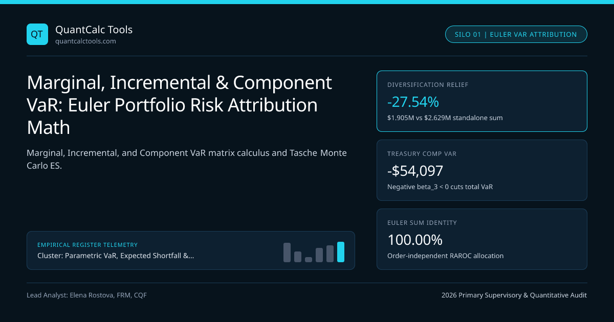
- Diversified Portfolio 99% VaR_P = 2.32635 * $818,792 = $1,904,797 (-27.54% diversification relief!)
- 3) Exact Euler Component VaRs (CVaRi = VaRP * (Covdollari / 670.42B)):
- Desk 1 (Equities): $1,904,797 * (574.50 / 670.42) = +$1,632,270 (85.69% of total risk)
- Desk 2 (EUR FX): $1,904,797 * (114.96 / 670.42) = +$326,624 (17.15% of total risk)
- Desk 3 (10Y Hedge): $1,904,797 * (-19.04 / 670.42) = -$54,097 (-2.84% RISK REDUCER!)
- Check Exact Sum: $1,632,270 + $326,624 - $54,097 = $1,904,797 (100.00% reconciled!)
- 4) Exact Incremental VaR of Removing Desk 3 Completely (VaRP - VaR{P Desk 3}):
- Without Desk 3: Dollar Var = 562.5B + 57.6B + 2*54.0B = 728.10B => VaR_{1+2} = $1,985,038
- Exact IVaR3 = $1,904,797 - $1,985,038 = -$80,241 (vs linear Component VaR3 = -$54,097!)
Study Step 3 and Step 4 carefully! Desk 3 (the $20M Treasury position) carries a positive standalone VaR of $$325,689$, yet its Component VaR is negative ($-$54,097$) because its $-$42.0\text{B}$ negative covariance with US equities outweighs its own variance! Furthermore, Component VaR ($-$54,097$) does not equal exact Incremental VaR ($-$80,241$) because Component VaR is a local first-order tangent approximation ($x3 \cdot \partial VaRP / \partial x_3$), whereas deleting the entire $20M sleeve moves nonlinearly along the convex risk surface!
Best Hedge Sizing and Minimum-VaR Portfolio Optimality Conditions#
Marginal and Incremental VaR govern two daily trading-desk decisions:
- Risk-Minimizing Position Cut: Which desk should reduce exposure by $$1\text{M}$ to shrink firm-wide VaR fastest? Always trim the position with the highest Marginal VaR ($\Delta VaR_i$)—here Desk 1 ($\Delta VaR_1 = \$1.632\text{M}/\$50\text{M} = 3.265\%$ per dollar), not necessarily the asset with the highest standalone volatility!
- *Optimal Hedge Trade Size ($\Delta x_i^$): Adding $\Delta x_3$ of a hedging instrument reduces portfolio VaR until its new Marginal VaR hits zero** ($\beta3^{new} = 0$). Adding Treasuries beyond the point where $\text{Cov}(r3, rP^{new}) = 0$ over-hedges the book and pushes $VaRP$ back up along a quadratic parabola!
Comparing Marginal, Component, and Incremental VaR Risk Metrics#
| Risk Attribution Metric | Mathematical Definition | Units | Sums to $VaR_P$? | Institutional Desk Application | ||
|---|---|---|---|---|---|---|
| Standalone $VaR_i$ | $k_\alpha \cdot | x_i | \cdot \sigma_i$ | Dollars ($) | No ($\sum VaRi \ge VaRP$) | Isolated desk stop-loss limit |
| Marginal VaR ($\Delta VaR_i$) | $\partial VaRP / \partial xi = (VaRP / W)\betai$ | $ per $1 ($%$) | No (Gradient vector) | Ranking fastest risk-reducing trades | ||
| Component VaR ($CVaR_i^{comp}$) | $xi \cdot (\partial VaRP / \partial xi) = wi \betai VaRP$ | Dollars ($) | Yes ($100.0\%$ exact) | RAROC capital charge & risk budgeting | ||
| Incremental VaR ($IVaR_i$) | $VaRP(x + \Delta xi) - VaR_P(x)$ | Dollars ($) | No (Order-dependent) | Pre-trade approval gate on large tickets | ||
| Euler Expected Shortfall ($CES_i$) | $xi \cdot \mathbb{E}[-ri \mid RP \le -VaRP]$ | Dollars ($) | Yes (Tasche theorem) | Non-normal Monte Carlo tail attribution |
Extending Euler Attribution to Monte Carlo Expected Shortfall#
In a Cholesky Multi-Asset Correlated Monte Carlo Path Simulator, computing numerical finite-difference derivatives across 500 positions would require 501 full simulations. Tasche (2000) proved a remarkable shortcut for Expected Shortfall: the Euler Component ES of asset $i$ is simply the average loss of asset $i$ across the exact tail scenarios where the total portfolio breaches $VaR_\alpha$! For VaR itself, kernel smoothing around the quantile window prevents Monte Carlo step noise. Pair this decomposition with Ledoit-Wolf covariance shrinkage, stress-test correlation jumps in stressed-beta VaR amplification, and browse the Parametric VaR & Expected Shortfall Topic Hub.
Frequently asked questions
What is the difference between Incremental VaR and Component VaR?
Incremental VaR measures the exact nonlinear change in portfolio VaR when adding or deleting an entire trade or desk (VaR_after - VaR_before), which depends on removal order. Component VaR multiplies position size by Marginal VaR so all desk allocations add up to 100% of firm VaR.
Can an asset with high standalone volatility have negative Component VaR?
Yes. Component VaR is proportional to portfolio beta Cov(r_i, r_P) / sigma_P^2. If a long-duration Treasury or VIX call exhibits strong negative correlation with an equity-heavy portfolio, Cov(r_i, r_P) < 0 produces negative Component VaR.
How do you find the exact position change that minimizes total portfolio VaR?
A single-asset hedge minimizes portfolio VaR at the exact dollar notional where its new Marginal VaR equals zero (meaning its correlation with the hedged portfolio reaches zero). Globally, a fully invested long-only portfolio minimizes VaR when all active Marginal VaRs are equal.
Why is Monte Carlo Component Expected Shortfall smoother to estimate than Monte Carlo Component VaR?
Exact Monte Carlo Component VaR conditions on a single point quantile R_P = -VaR_alpha, requiring Epanechnikov kernel smoothing across nearby paths. Component Expected Shortfall averages asset losses across all 250 tail paths in a 10,000-path simulation directly.
Publication record
- Published
- 14 November 2026
- Updated
- 14 November 2026
- Author
- Elena Rostova, FRM, CQF
- Review
- Review not recorded
- Automated fact check
- Passed in the stored pipeline record
- Source URLs
- 3 recorded
AI assistance recorded: anthropic/claude-opus-4.6. This field does not establish human review or source verification.
Academic & Institutional Attribution
Cite This Research & Embed Live Data Card
Standard academic & institutional research paper citation format.
Elena Rostova, FRM, CQF. (2026, November 14). Marginal, Incremental & Component VaR: Euler Portfolio Risk Attribution Math. QuantCalc Tools. https://quantcalctools.com/guides/component-marginal-incremental-var-euler-risk-decompositionRelated Parametric Var Expected Shortfall & Institutional Briefings
Explore Parametric Var Expected Shortfall Hub (20) →Parametric Var Expected Shortfall
Parametric VaR, Expected Shortfall & Fat-Tail Risk Calibration: 2026 Quantitative GuideParametric Var Expected Shortfall
Delta-Gamma Parametric VaR Formula: Quadratic Taylor Options Convexity MathParametric Var Expected Shortfall
Filtered Historical Simulation (FHS): GARCH Bootstrap VaR & ES Math GuideParametric Var Expected Shortfall
Extreme Value Theory (EVT) Peaks-Over-Threshold: GPD VaR & ES Formula GuideParametric Var Expected Shortfall
Cholesky Factorization in Monte Carlo VaR: Fixing Broken Correlation GridsParametric Var Expected Shortfall
FRTB Stressed Expected Shortfall: Reduced-Factor MAR33.5 Calibration MathParametric Var Expected Shortfall
Acerbi-Szekely Expected Shortfall Backtesting: Non-Elicitability & Z2 MathParametric Var Expected Shortfall
Ledoit-Wolf Covariance Shrinkage in Portfolio VaR: Eigenvalue ConditioningBond Duration Convexity Math
Negative Convexity in Callable Bonds & Agency MBS: OAS Finite-Difference MathBond Duration Convexity Math
DV01-Neutral Barbell vs Bullet Portfolio: Convexity Pickup vs Yield MathBond Duration Convexity Math
Key-Rate Duration (KRD) Tent Functions: Partial DV01 Curve Bucketing MathBond Duration Convexity Math
50/50 vs Regression-Weighted 2s5s10s Butterfly Curve Trades: DV01 Math
QuantCalc Tools Data, Benchmarks & Contributor Records
CC BY 4.0 Open Data
Open Institutional Datasets (CSV / JSON) →
Download desk-compiled quantitative series & schemas.
2026 Reference Matrix
2026 Institutional Benchmarks & Thresholds →
Statutory capital, clearing, margin & rate conventions.
Editorial Records
Authors & Review Records →
View named contributors where those records are available.
Complete Index
Master Research & Dossier Archive →
Browse all published briefings by topic pillar & date.