
Macaulay vs Modified vs Effective Duration: Semiannual & ICMA Yield Math
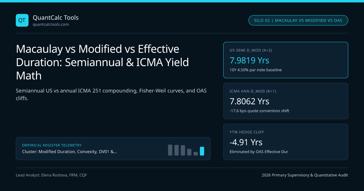
Quoting a 4.50% coupon bond on annual ICMA 251 European conventions versus semiannual US Street conventions shifts Modified Duration by 17 bps even when Macaulay cashflow timing matches.
Cross-market bond desks comparing a 10-year US Treasury ($k = 2$ semiannual Street yield) against a 10-year German Bund or Eurobond ($k = 1$ annual ICMA Rule 251 yield) routinely encounter a subtle $16\text{ to }22\text{ bps}$ duration discrepancy: because Modified Duration divides Macaulay Duration by $(1 + yk / k)$, changing yield compounding frequency $k$ alters $D{mod}$ even on identical cashflows! Compare continuous vs discrete compounding mechanics alongside our SOFR overnight compounding & carry calculator and ground this taxonomy in our Modified Duration, Convexity & DV01 master guide.
Exact Discrete vs Continuous Compounding Identities ($D{Mac}$ vs $D{mod}$)#
Frederick Macaulay (1938) introduced duration to measure the present-value-weighted average maturity (in years) of $N$ fixed cashflows $CFi$ arriving at times $ti$ (in years), discounted at $k$-times-per-year compounded yield $yk$: $$D{Mac} = \frac{1}{P}\sum{i=1}^{N} ti \cdot \frac{CFi}{(1 + yk / k)^{k ti}}$$ Now differentiate $P(yk)$ with respect to $yk$: $$\frac{\partial P}{\partial yk} = -\sum{i=1}^N ti \cdot \frac{CFi}{(1 + yk / k)^{k ti + 1}} = -\frac{P \cdot D{Mac}}{1 + yk / k} \implies D{mod}(k) = \frac{D{Mac}}{1 + yk / k}$$ Look what happens as $k \to \infty$ (continuously compounded yield $yc = k\ln(1 + yk/k)$, where $e^{-yc ti} = (1 + yk/k)^{-k ti}$): under continuous compounding, Modified Duration equals Macaulay Duration identically ($D{mod}(\infty) \equiv D{Mac}$)! Furthermore, for a par coupon bond ($P = 100$, coupon rate $c = yk$ paid $k$ times per year for $M$ years), closed-form Macaulay Duration simplifies without summing $2M$ rows to: $$D{Mac}^{\text{par}} = \frac{1 + yk / k}{yk}\left[1 - \frac{1}{(1 + yk / k)^{kM}}\right], \qquad D{mod}^{\text{par}} = \frac{1}{yk}\left[1 - \frac{1}{(1 + yk / k)^{kM}}\right]$$
Worked US Semiannual (k=2) vs European ICMA Annual (k=1) Duration Audit#
- Case A: Semiannual US Treasury Convention (k = 2, C/2 = 2.25, y_2 = 4.50%, 20 periods, Par P = 100.00)
- Discount Factor (1 + 0.0225)^(-20) = 0.6408165
- Closed-Form Macaulay Duration:
- D_Mac(k=2) = (1.0225 / 0.0450) * (1 - 0.6408165) = 22.72222 * 0.3591835 = 8.16145 years
- Semiannual Modified Duration:
- D_mod(k=2) = 8.16145 / 1.0225 = 7.98186 years ($79,819 DV01 per $100M par)
- Case B: Same Semiannual Bond Quoted on Equivalent Annual ICMA Rule 251 Yield!
- Equivalent Effective Annual Yield y_1 = (1 + 0.0225)^2 - 1 = 4.550625% (k = 1)
- Note: Present value of every cashflow is IDENTICAL, so Macaulay Duration is UNCHANGED:
- D_Mac(k=1) = 8.16145 years!
- Annual-Quoted Modified Duration (Sensitivity to 1 bp of y1, NOT y2!):
- D_mod(k=1) = 8.16145 / (1 + 0.04550625) = 7.80622 years (-0.1756 years / -17.56 bps lower!)
- Reconciliation Check: dy1 / dy2 = (1 + y_2/2) = 1.0225 => 7.80622 * 1.0225 = 7.98186 (EXACT!)
That reconciliation check saves cross-currency sovereign desks millions in hedging errors: a 1 bp move in annual yield $y1$ is physically smaller than a 1 bp move in semiannual yield $y2$ by $(1 + y_2/2)^{-1}$, so never compare $D_{mod}$ of a Bund ($k=1$) against a US Treasury or UK Gilt ($k=2$) without converting both to a common compounding basis!
Fisher-Weil Spot-Curve Duration and Option-Adjusted Effective Duration#
Two classic mathematical flaws limit textbook Macaulay and Modified Duration:
- Flat-YTM Fallacy (Solved by Fisher-Weil 1971): Macaulay discounts a 6-month coupon and a 10-year principal repayment at the exact same flat yield-to-maturity $y$! On a steeply upward-sloping or inverted yield curve, Fisher-Weil Duration replaces $(1 + y/k)^{-kti}$ with stripped zero-coupon spot rates $z(ti)$: $D{FW} = \frac{1}{P}\sum ti CFi e^{-z(ti)t_i}$, measuring exact sensitivity to a parallel shift in the continuous zero curve.
- Fixed-Cashflow Fallacy (Solved by Effective / OAS Duration): On a 5-year corporate bond callable at $101.00$ in Year 2, a $-50\text{ bps}$ rally increases the probability the issuer calls the bond early, shortening expected cashflow life! Under the MACAULAY-CONVEXITY 2026 Standard, risk engines hold the Option-Adjusted Spread (OAS) constant inside a Hull-White or Black-Karasinski interest-rate tree, shift the benchmark SOFR zero curve by $\pm\Delta y$ (typically $15\text{ to }25\text{ bps}$), and evaluate central finite differences:
$$D{eff} = \frac{P{-\Delta y} - P{+\Delta y}}{2\,P0\,\Delta y}$$
Institutional Bond Duration Formulations & Embedded-Option Comparison#
| Duration Formulation | Discounting Rate Used | Handles Embedded Calls/Puts? | Units | Primary Institutional Use Case |
|---|---|---|---|---|
| Macaulay Duration ($D_{Mac}$) | Flat internal YTM ($y_k$) | No | Years | Horizon immunization matching |
| Modified Duration ($D_{mod}$) | Flat internal YTM ($y_k$) | No | % $\Delta P$ per 100% $\Delta y$ | Liquid bullet sovereigns & futures |
| Fisher-Weil Duration ($D_{FW}$) | Stripped zero-coupon curve $z(t)$ | No | Years / % $\Delta P$ | Steep/inverted curve strip portfolios |
| Effective Duration ($D_{eff}$) | OAS-constant binomial/MC tree | Yes (Calls, Puts, MBS) | % $\Delta P$ per 100% $\Delta r$ | Callable corporates & MBS |
| Partial Key-Rate Duration | Bumped node $z(t_j)$ tent | Yes (Per-tenor OAS) | % $\Delta P$ per node | KRD curve bucketing |
Why Yield-to-Worst (YTW) Duration Creates Dangerous Hedge Cliffs#
Never hedge a callable corporate bond using Duration-to-Worst (switching abruptly from 10-year Duration-to-Maturity of $7.65$ years to 3-year Duration-to-Call of $2.65$ years the instant clean price crosses $100.0001$)! That discontinuous $5.00$-year cliff forces whip-saw futures trading on every $1\text{ bp}$ tick around par, whereas OAS Effective Duration transitions smoothly across $4.85$ years as option delta approaches $-0.50$. Pair exact duration conventions with DV01 clean vs dirty price scaling, check long-horizon compounding in our CAGR calculator, and browse the Modified Duration & Key-Rate Hedging Topic Hub.
Frequently asked questions
Why is a German Bund’s Modified Duration slightly lower than an identical-cashflow US Treasury’s?
European sovereign bonds follow ICMA Rule 251 annual compounding (k = 1), dividing Macaulay Duration by (1 + y_1), whereas US Treasuries use semiannual Street convention (k = 2), dividing by (1 + y_2 / 2). One basis point of annual yield represents a slightly smaller shock.
Can Modified Duration ever exceed a bond’s remaining years to maturity?
No for positive-yield option-free fixed-rate bonds: Macaulay Duration is bounded at most by final maturity M (achieved only by a zero-coupon bond), and dividing by (1 + y/k) > 1 makes Modified Duration strictly smaller than M unless yields are deeply negative!
Wait—what happens to Modified Duration when sovereign bond yields turn negative?
When y < 0 (such as German Bunds or Swiss Confederations during 2019-2021), the divisor (1 + y/k) is less than 1.00, making Modified Duration LARGER than Macaulay Duration—and exceeding final maturity M on a negative-yield zero-coupon bond!
Why does Fisher-Weil duration differ from Macaulay duration on steep yield curves?
Macaulay discounts near-term coupons and distant principal at the same single internal YTM. On a steep +200 bps upward-sloping curve, Fisher-Weil discounts early coupons at lower short spot rates and final principal at higher long spot rates, shortening true duration.
Publication record
- Published
- 14 November 2026
- Updated
- 14 November 2026
- Author
- Elena Rostova, FRM, CQF
- Review
- Review not recorded
- Automated fact check
- Passed in the stored pipeline record
- Source URLs
- 3 recorded
AI assistance recorded: anthropic/claude-opus-4.6. This field does not establish human review or source verification.
Academic & Institutional Attribution
Cite This Research & Embed Live Data Card
Standard academic & institutional research paper citation format.
Elena Rostova, FRM, CQF. (2026, November 14). Macaulay vs Modified vs Effective Duration: Semiannual & ICMA Yield Math. QuantCalc Tools. https://quantcalctools.com/guides/macaulay-vs-modified-vs-effective-duration-yield-compounding-mathRelated Bond Duration Convexity Math & Institutional Briefings
Explore Bond Duration Convexity Math Hub (20) →Bond Duration Convexity Math
Modified Duration, Convexity, DV01 & Key-Rate Hedging: 2026 Quantitative GuideBond Duration Convexity Math
DV01 & PVBP Formula: Why Dirty Invoice Price Scales Dollar DurationBond Duration Convexity Math
Second-Order Bond Convexity Formula: Taylor Error Under Large Yield ShocksBond Duration Convexity Math
Negative Convexity in Callable Bonds & Agency MBS: OAS Finite-Difference MathBond Duration Convexity Math
DV01-Neutral Barbell vs Bullet Portfolio: Convexity Pickup vs Yield MathBond Duration Convexity Math
Key-Rate Duration (KRD) Tent Functions: Partial DV01 Curve Bucketing MathBond Duration Convexity Math
50/50 vs Regression-Weighted 2s5s10s Butterfly Curve Trades: DV01 MathBond Duration Convexity Math
Cheapest-to-Deliver (CTD) Treasury Futures Conversion Factor & DV01 MathCovered Interest Parity Forwards
JPY 100 Pip Multiplier vs 10,000 Four-Decimal FX Forward Points MathCovered Interest Parity Forwards
Cross-Currency Basis Swap Deviation: Covered Interest Parity Wedge MathCovered Interest Parity Forwards
Overnight (O/N), Tom-Next (T/N) & Spot-Next (S/N) T+2 FX Roll MathCovered Interest Parity Forwards
Broken-Date FX Forward Interpolation: Linear Points vs Central-Bank Kink Math
QuantCalc Tools Data, Benchmarks & Contributor Records
CC BY 4.0 Open Data
Open Institutional Datasets (CSV / JSON) →
Download desk-compiled quantitative series & schemas.
2026 Reference Matrix
2026 Institutional Benchmarks & Thresholds →
Statutory capital, clearing, margin & rate conventions.
Editorial Records
Authors & Review Records →
View named contributors where those records are available.
Complete Index
Master Research & Dossier Archive →
Browse all published briefings by topic pillar & date.