
Ralph Vince Optimal f & Terminal Wealth Relative (TWR): Empirical Sizing Math
Real trading logs contain partial exits, scratch trades, and fat-tailed outliers rather than two neat binary outcomes; derive Ralph Vince Optimal f and largest-loss contract scaling.
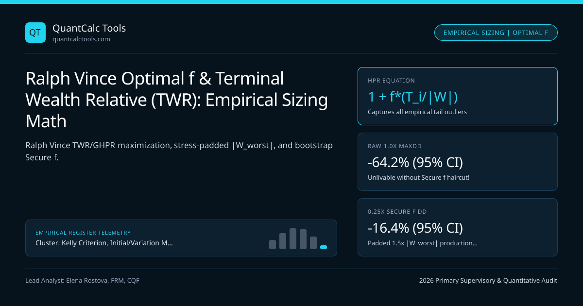
What happens when you export a 400-trade execution log from MT5 or TradingView and try to plug it into the textbook two-state discrete binomial Kelly formula $p - q/R$? You immediately discover that real trade logs are multi-modal empirical distributions—containing +0.1R scratch breakevens, -1.0R normal stops, -2.8R overnight gap losses, and +11.5R home-run runners! Reducing 400 rich empirical P&L outcomes to just two averages (Avg Win and Avg Loss) throws away crucial tail kurtosis! In Portfolio Management Formulas (1990) and The Mathematics of Money Management (1992), Ralph Vince formulated Empirical Optimal f—maximizing exact Geometric Mean Holding Period Return (GHPR) directly over all $N$ historical dollar P&L outcomes normalized by the Largest Historical Loss (|W_worst|)! Benchmark parametric vs empirical fractions in our Kelly Criterion Calculator and Kelly, Margin & Liquidation Hub.
Exact Ralph Vince HPR, TWR, GHPR, and Dollar-Per-Contract Equations#
Let $\{T1, T2, \dots, TN\}$ be the realized net dollar P&L per 1 contract (or per 1 lot, after commissions and slippage) across $N$ historical trades, with strictly negative worst single-trade loss $W{\text{worst}} = \mini Ti < 0$ (so $|W{\text{worst}}| > 0$). For any candidate risk fraction $f \in (0, 1)$, Vince defines trade $i$'s **Holding Period Return (`HPRi(f))**, cumulative **Terminal Wealth Relative (TWR(f))**, and contract count Contracts` as:
- 1. Single-Trade Holding Period Return (Normalized by Worst Loss |W_worst| > 0):
- HPRi(f) = 1 + f * ( Ti / |W_worst| ) for f in (0, 1)
- (Note: If f = 1.00 and Wworst recurs, HPRworst = 1 + 1.0*(-1) = 0.00 -> Instant 100% Wipeout!)
- 2. Terminal Wealth Relative & Geometric Mean HPR across N Trades:
- TWR(f) = Product{i=1..N} HPRi(f) = Product{i=1..N} [ 1 + f * (Ti / |W_worst|) ]
- GHPR(f) = [ TWR(f) ]^(1 / N) <=> Maximize L(f) = (1 / N) * Sum{i=1..N} ln( 1 + f * (Ti / |W_worst|) )
- 3. First-Order Brent/Newton Root for Optimal f* (Unique Concave Peak when Mean(T_i) > 0):
- L'(f) = Sum{i=1..N} [ Ti / ( |W_worst| + f * T_i ) ] = 0
- 4. Converting Optimal f* (or Diluted c * f*) into Live Account Dollar Divisor & Contracts:
- DollarUnitperContract = |Wworst| / fused => Contracts = floor( AccountEquity / DollarUnitper_Contract )
- Worked 5-Trade Skewed Empirical Audit (Per-Contract PnLs: [+$900, -$300, +$1,800, -$600, -$300]):
- Mean PnL = +$300/trade (> $0 positive edge!), Worst Loss |W_worst| = $600 (Trade #4):
- Evaluate TWR(f) = (1 + 1.5f) * (1 - 0.5f)^2 * (1 + 3.0f) * (1 - 1.0f):
- At f = 0.15 : TWR = (1.225)(0.8556)(1.450)*(0.850) = 1.2919 (GHPR = 1.0526 => +5.26%/trade)
- At f = 0.236: TWR = 1.3268 (EXACT PEAK Optimal f* = 23.6% => GHPR = 1.0582 => +5.82%/trade)
- At f = 0.50 : TWR = (1.750)(0.5625)(2.500)*(0.500) = 1.2305 (Over-betting drops TWR & risks -50% on 1 repeat of -$600!)
- Practical Diluted Quarter-Optimal-f (f_used = 0.25 * 0.236 = 0.059):
- Dollar_Unit = $600 / 0.059 = $10,169 per contract -> Trade 9 contracts on a $100,000 account!
Single-Trade Tail Shock Under Undiluted Optimal f Versus Quarter-Vince Sizing#
Look closely at Equation 4 (Dollar_Unit = |W_worst| / f_used): if Optimal f* = 0.236, trading undiluted f* = 0.236 means the very next time a loss equal to your historical worst loss -$600 occurs, your account instantly drops -23.6% on ONE single trade—and if the future worst loss is 1.5x worse than your historical sample (-$900), you lose -35.4% in one afternoon!
Why Sample |W_worst| Is Biased Downward & How Extreme Value Theory Fixes It#
Notice a subtle statistical flaw in raw Ralph Vince Optimal f: the denominator |W_worst| = max_i(-T_i) is a sample maximum over finite $N$ trades! By Extreme Value Theory, the worst loss over your next $1{,}000$ live trades exceeds the worst loss over your first $100$ backtested trades with $90.9\%$ probability ($1000 / (100 + 1000)$)! Institutional systematic desks apply two mandatory upgrades before turning Optimal f live:
- Tail-Padded
|W_stress|: Replace raw sample|W_worst|withmax(1.5 * |W_worst|, Expected_Shortfall_99.5%)modeled via Cornish-Fisher / Generalized Pareto tails. - Leo Zamansky & David Stendahl's
Secure f: MaximizeGHPR(f)across10,000block-bootstrapped resamples of $\{Ti\}$ subject to **95th-percentile Maximum Drawdown $\le D{\text{max}}$** (which seamlessly bridges Vince's empirical framework to drawdown-constrained fractional Kelly!).
Comparison of Position-Sizing Algorithms Across Skewed Empirical Trade Logs#
Compare how four sizing methods handle fat-tailed trade distributions (N = 250 trades, +0.38R expectancy, 1 outlier -4.2R gap loss):
| Position-Sizing Method | Uses Full $N$-Trade Distribution? | Accounts for -4.2R Outlier Gap? | Typical Undiluted Drawdown | Institutional Production Adaptation | ||||
|---|---|---|---|---|---|---|---|---|
2-State Binomial Kelly (p - q/R) | No (only p & AvgW/AvgL) | No! (Hides -4.2R inside AvgL!) | $55\%\text{--}85\%$ (Can hit ruin on gap!) | Dangerous on fat-tailed gap logs | ||||
Continuous Merton (mu / sigma^2) | Uses 1st & 2nd moments | Partial (via inflated $\sigma^2$) | $45\%\text{--}65\%$ | Shrink to 0.25x–0.50x (Half-Kelly) | ||||
Ralph Vince Raw Optimal f | Yes (Every single $T_i$!) | Yes (Anchored to ` | W_worst | `!) | $50\%\text{--}75\%$ (Unacceptable raw!) | Dilute to 0.20x–0.30x + pad ` | W_worst | ` |
Bootstrap Secure f (Zamansky) | Yes (Full path resamples) | Yes (`1.5x | W_worst | ` + streaks) | Capped at Mandated $15\%\text{--}20\%$! | Best-in-class empirical single-system sizing |
Always Verify Dollar_Unit >= Exchange Initial Margin!#
Suppose Secure f outputs Dollar_Unit = $12,000 per E-mini S&P (ES) contract, while CME SPAN 2 Speculator Initial Margin is $15,400 per contract! Exchange Initial Margin is a hard physical floor: your executable divisor is max(Dollar_Unit_Secure_f, 1.5 * Exchange_IM_per_Lot). Cross-verify risk of ruin in Markov absorption vs fixed-fractional ruin math and CAGR volatility drag.
Frequently asked questions
When does Ralph Vince Optimal f give the EXACT same answer as the textbook Discrete Kelly formula?
Whenever your empirical trade log consists solely of two discrete outcomes (+b dollars on fraction p of trades, and -a dollars on fraction q = 1 - p of trades)! In that binary case, |W_worst| = a, and setting Vince’s derivative L’(f) = p*(b/a)/(1 + f*b/a) - q/(1 - f) = 0 solves identically to f* = p - q / (b/a)!
Should I feed percentage returns or 1-contract dollar PnLs into Optimal f for futures and FX?
For futures and FX lots, feed price-normalized 1-contract constant-point/percentage PnLs (or constant $100k notional PnLs)! Why? Because a -$500 point move when Gold was $1,200/oz (-4.2%) is twice as severe in percentage volatility as a -$500 move when Gold is $2,600/oz (-1.9%)—always normalize T_i to current contract price!
What is Ralph Vince’s "Leverage Space Portfolio Model" (2009)?
Vince extended univariate Optimal f to M simultaneous trading systems by maximizing joint N-period geometric HPR over the M-dimensional hypercube f = (f_1, ..., f_M) in [0, 1]^M subject to a global path drawdown probability constraint—the exact non-parametric empirical cousin of Multi-Asset Drawdown-Constrained Kelly!
How does Ryan Jones’s "Fixed Ratio" position sizing differ from Ralph Vince’s Fixed Fractional Optimal f?
Fixed Fractional (Optimal f) scales contract count linearly with equity (Contracts = Equity / Dollar_Unit), whereas Ryan Jones’s Fixed Ratio scales contract count with the SQUARE ROOT of accumulated profits via parameter Delta—growing faster on small accounts and automatically de-leveraging as equity becomes large!
Publication record
- Published
- 13 November 2026
- Updated
- 14 November 2026
- Author
- Elena Rostova, FRM, CQF
- Review
- Review not recorded
- Automated fact check
- Passed in the stored pipeline record
- Source URLs
- 4 recorded
AI assistance recorded: anthropic/claude-opus-4.6. This field does not establish human review or source verification.
Academic & Institutional Attribution
Cite This Research & Embed Live Data Card
Standard academic & institutional research paper citation format.
Elena Rostova, FRM, CQF. (2026, November 14). Ralph Vince Optimal f & Terminal Wealth Relative (TWR): Empirical Sizing Math. QuantCalc Tools. https://quantcalctools.com/guides/ralph-vince-optimal-f-empirical-trade-distribution-largest-lossRelated Kelly Margin Leverage Sizing & Institutional Briefings
Explore Kelly Margin Leverage Sizing Hub (20) →Kelly Margin Leverage Sizing
Kelly Criterion, Initial/Variation Margin & Liquidation Math: 2026 GuideKelly Margin Leverage Sizing
Short Naked Option Margin Math: Reg T 20%/10% Rule & Gamma Crash ExpansionKelly Margin Leverage Sizing
Repo Haircut, Rehypothecation Multiplier & Leveraged Bond Carry MathKelly Margin Leverage Sizing
Black-Litterman Posterior Expected Return & Bayesian Kelly Sizing MathKelly Margin Leverage Sizing
Guaranteed Stop-Loss Order (GSLO) Premium vs Gap Slippage & Option MathKelly Margin Leverage Sizing
Discrete Binomial Kelly Criterion: Win Rate & Asymmetric Payoff ProofKelly Margin Leverage Sizing
Continuous Merton-Kelly Leverage ((mu - r_f)/sigma^2) & Half-Kelly MathKelly Margin Leverage Sizing
Multi-Asset Kelly Portfolio Sizing: Inverse-Covariance & Shrinkage MathMarket Insights
UBS downgrades DraftKings stock rating on valuation concernsMarket Insights
Bulls vs. Bears: NVIDIA sparks valuation debate as stock nears six-month lowIPO and Funding
Anthropic IPO Valuation Could Be Slashed in Half to $1T After AI Stock Rout: ReportIPO and Markets
Anthropic's $1.5 trillion IPO valuation in doubt after tech sell-off hammers the market
QuantCalc Tools Data, Benchmarks & Contributor Records
CC BY 4.0 Open Data
Open Institutional Datasets (CSV / JSON) →
Download desk-compiled quantitative series & schemas.
2026 Reference Matrix
2026 Institutional Benchmarks & Thresholds →
Statutory capital, clearing, margin & rate conventions.
Editorial Records
Authors & Review Records →
View named contributors where those records are available.
Complete Index
Master Research & Dossier Archive →
Browse all published briefings by topic pillar & date.