
Discrete Binomial Kelly Criterion: Win Rate & Asymmetric Payoff Proof
Textbook f* = p - q/b assumes losing 100% of staked capital on every losing trade; derive the exact generalized asymmetric stop-loss Kelly formula f* = p/a - q/b for real financial markets.
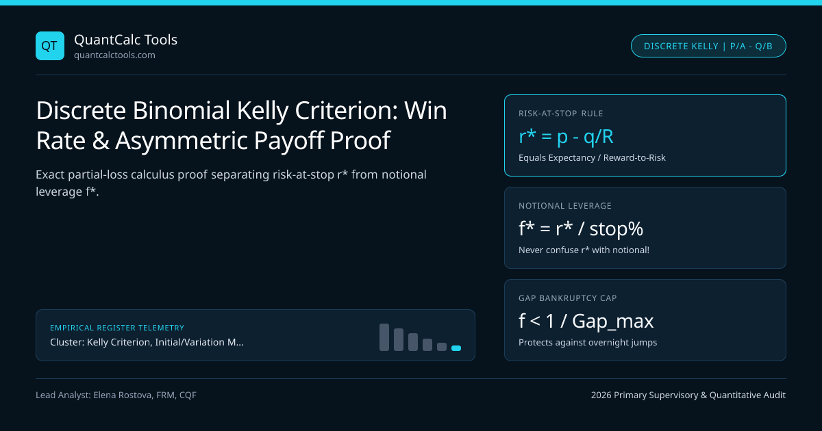
When systematic traders first transcribe John Kelly's 1956 Bell Labs paper (A New Interpretation of Information Rate) into trading code, $90\%$ copy the casino binary formula *$f^ = p - \frac{q}{b}$** and wonder why it outputs f* = 0.25 (25% of total equity), completely unsure whether 25% means "put 25% of portfolio notional into Apple stock" or "risk 25% of portfolio equity to my stop-loss"! Confusing those two numbers by a factor of $10\times$ on a -2.5% stop-loss trade is the #1 position-sizing error in retail and emerging-quant trading! Verify exact both-convention outputs in our Kelly Criterion Calculator, inspect the Half-Kelly Portfolio Leverage Engine, and anchor in our Kelly, Margin & Liquidation Hub.
Exact First-Principles Calculus Proof: Generalized Partial-Loss Kelly ($f^* = \frac{p}{a} - \frac{q}{b}$)#
In a casino coin toss or expiring binary option, a losing bet forfeits $100\%$ of staked capital ($a = 1.00$). In liquid financial markets, a trade allocated fraction $f$ of total portfolio equity either gains $+b$ per dollar allocated with probability $p$ OR hits a stop-loss losing $-a$ per dollar allocated ($0 < a \le 1$) with probability $q = 1 - p$. Write single-trial expected logarithmic wealth growth $G(f) = \mathbb{E}[\ln(W1 / W0)]$ and set its first derivative $G'(f) = 0$:
- Log-Growth Objective : G(f) = p * ln(1 + f * b) + q * ln(1 - f * a)
- First Derivative = 0 : G'(f) = [ p * b / (1 + f * b) ] - [ q * a / (1 - f * a) ] = 0
- Cross-Multiply & Solve : pb(1 - fa) = qa(1 + fb) => pb - qa = fab(p + q) = fa*b
- 1. Optimal Capital Allocation Fraction (f*_notional) :
- f_notional = (p b - q * a) / (a * b) = (p / a) - (q / b) = Expected_Edge / (a * b)
- 2. Optimal Capital-at-Risk to Stop-Loss (r_risk = f_notional * a, letting R = b / a = Reward-to-Risk Ratio!):
- r_risk = f_notional * a = p - (q / R) <-- Classic Kelly gives RISK-AT-STOP %, NOT notional %!
- Worked Swing-Trade Proof (Win Rate p = 45.0%, Loss Rate q = 55.0%, Stop-Loss a = -2.0%, Target Gain b = +6.0% => R = 3.0):
- 1. Capital-at-Risk to Stop (r*_risk) = 0.45 - (0.55 / 3.0) = 0.45 - 0.1833 = 26.67% risk-to-stop (Full Kelly!)
- Institutional Quarter-Kelly Risk-at-Stop (0.25 * r*) = 6.67% of equity risked to the -2.0% stop (or 1–2% Desk Cap!)
- 2. Notional Capital Allocation (f_notional = r_risk / a):
- Full Kelly Notional = 0.2667 / 0.02 = 13.33x Leverage! | Quarter-Kelly Notional = 3.33x Leverage!
- 3. Check Second Derivative Concavity: G''(f) = -pb^2/(1+fb)^2 - qa^2/(1-fa)^2 < 0 strictly (Unique Global Max!)
Read Equations 1 and 2 side-by-side—that single algebraic identity resolves decades of confusion:
- Classic $p - q/R$ (where $R = \text{Avg Win} / \text{Avg Loss}$) tells you the fraction of account equity risked IF your stop-loss is hit ($r^*_{\text{risk}}$)!
- Dividing $r^_{\text{risk}}$ by percentage stop distance $a$ gives notional position leverage* $f^_{\text{notional}} = r^_{\text{risk}} / a$!
Why Gap Slippage Beyond -a Shatters Un-Haircutted Discrete Kelly!#
Look closely at the logarithm $\ln(1 - f \cdot a)$ inside the discrete Kelly objective: if your stop-loss is set at $a = 2.0\%$ and you lever notional to $f = 13.33\times$ (so $f \cdot a = 26.67\%$ loss on a normal stop), what happens if an earnings gap or weekend FX jump opens -8.0% against you (4x your planned -2.0% stop)? At $f = 13.33\times$ notional leverage, an $-8.0\%$ overnight gap inflicts $13.33 \times (-8.0\%) =$ -106.7% total account bankruptcy ($\ln(1 - 1.067)$ is undefined—total ruin)! Whenever actual worst-case gap loss $a{\max}$ exceeds planned stop $a$, true discrete Kelly is bounded strictly below $1 / a{\max}$—formalized in Ralph Vince Optimal f largest-loss scaling!
Breakeven Win-Rate & Half-Kelly Risk-at-Stop Matrix Across Payoff Asymmetry ($R = b/a$)#
Verify how win rate $p$ and net reward-to-risk ratio $R$ interact to determine *Half-Kelly Risk-at-Stop ($0.5 r^$)** across four archetypal trading styles:
| Strategy Archetype | Win Rate ($p$) | Net Reward / Risk ($R = b/a$) | Breakeven Win Rate ($1/(1+R)$) | Expectancy per $1 Risked | Full-Kelly Risk ($r^*$) | *Half-Kelly Risk ($0.5 r^$)** |
|---|---|---|---|---|---|---|
| Mean-Reversion Scalp | $65.0\%$ | $1.00 : 1$ | $50.0\%$ | $+\$0.30$ | $30.0\%$ | $15.0\%$ (Cap at $2\%$ for gap risk!) |
| Swing Pullback Desk | $50.0\%$ | $2.00 : 1$ | $33.3\%$ | $+\$0.50$ | $25.0\%$ | $12.5\%$ |
| Breakout Momentum | $38.0\%$ | $3.00 : 1$ | $25.0\%$ | $+\$0.52$ | $17.3\%$ | $8.67\%$ |
| Macro Trend / Tail CTA | $25.0\%$ | $6.00 : 1$ | $14.3\%$ | $+\$0.75$ | $12.5\%$ | $6.25\%$ |
| Zero-Edge Overtrader | $40.0\%$ | $1.45 : 1$ | $40.8\%$ | $-\$0.02$ | $-1.38\% \to 0\%$ | $0.00\%$ (Negative expectancy!) |
The Equal-Expectancy Paradox: Why r* = Expectancy / R!#
Look at the algebraic gem revealed in the chart above: since trade expectancy per dollar risked is $ER = p R - q$, rewrite discrete Kelly as: $$r^*{\text{risk}} = p - \frac{q}{R} = \frac{p R - q}{R} = \frac{\text{Expectancy}}{R}$$ Two traders with the exact same +$0.50 expectancy per dollar risked DO NOT bet the same fraction! A p = 75%, R = 1 system has r* = 0.50 / 1 = 50%, whereas a p = 25%, R = 5 trend-follower has r* = 0.50 / 5 = 10% because 25% win-rate strategies naturally endure 12-to-18 consecutive losing trades!
Connecting Discrete Binomial Kelly to Continuous Merton Diffusion & Lot Sizing#
When trading continuous return distributions rather than fixed stop/target brackets, transition smoothly to continuous Merton-Kelly leverage $\mu / \sigma^2$ and drawdown-constrained fractional Kelly, convert r*_risk into exact currency lots via FX pip-value lot sizing math, and verify margin limits on UK FCA regulated venues in our broker lookup directory.
Frequently asked questions
Why does John Kelly’s original 1956 paper connect optimal betting to Claude Shannon’s Information Theory?
Kelly examined a gambler receiving a noisy binary communication channel with crossover error probability q = 1 - p! On even-money odds (b = a = 1), optimal bet f* = p - q = 2p - 1 yields maximum asymptotic exponential growth rate ln(2) + p*ln(p) + q*ln(q)—which is literally Shannon’s channel capacity in nats per transmission!
What happens if my strategy has a positive win rate (say 60%) but f* = p - q/R comes out negative?
A negative Kelly fraction (for example, p = 60%, q = 40%, R = 0.50 -> r* = 0.60 - 0.80 = -0.20) proves your strategy has NEGATIVE mathematical expectancy (0.60*0.50 - 0.40*1 = -$0.10 per $1 risked)! Unless you can take the opposite side of the trade (excluding transaction costs), optimal allocation is strictly f* = 0.
How do brokerage commissions and bid-ask spread change b and a in the Kelly formula?
Suppose round-trip spread plus commission equals c = 0.15% of notional on a 1.0% stop / 2.0% target trade. Effective net win shrinks to b_net = 2.0% - 0.15% = 1.85%, while effective net loss widens to a_net = 1.0% + 0.15% = 1.15%—cutting R from 2.00 down to 1.61 and slashing Full Kelly by over 35%!
Why do professional prop desks risk 0.5% to 2.0% per trade when Half-Kelly says 6% to 12%?
Three practical constraints: (1) Traders hold 5 to 15 correlated open positions simultaneously (so 10 positions x 1% risk = 10% aggregate correlated stop risk!); (2) Win rate p and payoff R drift across market regimes; and (3) Prop/institutional mandates cap maximum peak-to-trough drawdown at 10%–15%, requiring ~0.15x–0.25x Kelly.
Publication record
- Published
- 13 November 2026
- Updated
- 14 November 2026
- Author
- Elena Rostova, FRM, CQF
- Review
- Review not recorded
- Automated fact check
- Passed in the stored pipeline record
- Source URLs
- 4 recorded
AI assistance recorded: anthropic/claude-opus-4.6. This field does not establish human review or source verification.
Academic & Institutional Attribution
Cite This Research & Embed Live Data Card
Standard academic & institutional research paper citation format.
Elena Rostova, FRM, CQF. (2026, November 14). Discrete Binomial Kelly Criterion: Win Rate & Asymmetric Payoff Proof. QuantCalc Tools. https://quantcalctools.com/guides/discrete-binomial-kelly-criterion-win-rate-payoff-asymmetry-proofRelated Kelly Margin Leverage Sizing & Institutional Briefings
Explore Kelly Margin Leverage Sizing Hub (20) →Kelly Margin Leverage Sizing
Kelly Criterion, Initial/Variation Margin & Liquidation Math: 2026 GuideKelly Margin Leverage Sizing
Continuous Merton-Kelly Leverage ((mu - r_f)/sigma^2) & Half-Kelly MathKelly Margin Leverage Sizing
Multi-Asset Kelly Portfolio Sizing: Inverse-Covariance & Shrinkage MathKelly Margin Leverage Sizing
Drawdown-Constrained Fractional Kelly: Exact Probability of X% Loss MathKelly Margin Leverage Sizing
UK FCA COBS 22.5 & ESMA Retail Leverage Caps & 50% Margin Close-Out MathKelly Margin Leverage Sizing
Isolated Margin vs Cross-Margin Liquidation & Bankruptcy Price FormulasKelly Margin Leverage Sizing
CME SPAN 2 Historical VaR Margin & Futures Maintenance Top-Up MathKelly Margin Leverage Sizing
ISDA SIMM v2.6 Uncleared OTC Initial Margin: Delta, Vega & Curvature MathRegulatory Compliance
Financial Stability Board to launch hedge fund leverage data consultation - Traders UnionMarket Insights
Rayonier jumped after earnings. Why we still see upside for the timber REITMarket Insights
10-year Treasury yield jumps back above 5% as oil gains and more Fed rate hikes expectedVenture Capital
Ukrainian defense tech startup hits $6 billion valuation as investors bet on battle-tested drones
QuantCalc Tools Data, Benchmarks & Contributor Records
CC BY 4.0 Open Data
Open Institutional Datasets (CSV / JSON) →
Download desk-compiled quantitative series & schemas.
2026 Reference Matrix
2026 Institutional Benchmarks & Thresholds →
Statutory capital, clearing, margin & rate conventions.
Editorial Records
Authors & Review Records →
View named contributors where those records are available.
Complete Index
Master Research & Dossier Archive →
Browse all published briefings by topic pillar & date.