
Parametric Var Expected Shortfall
Extreme Value Theory (EVT) Peaks-Over-Threshold: GPD VaR & ES Formula Guide
By the Pickands-Balkema-de Haan theorem, tail losses exceeding a high threshold converge to a Generalized Pareto Distribution, enabling closed-form 99.9% VaR and Expected Shortfall extrapolation.
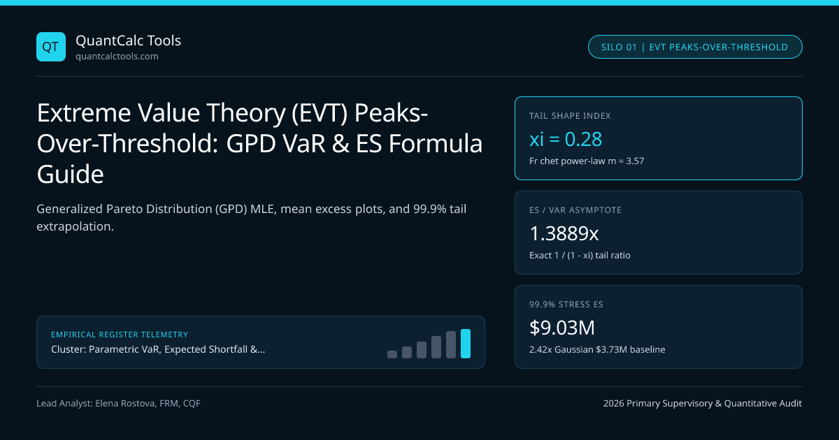
Fitting a distribution to 100% of daily portfolio returns forces the 95% quiet-market center to dictate the 0.5% catastrophic crash tail—a compromise that fails whenever flash crashes, currency de-pegs, or sovereign defaults obey power-law physics distinct from everyday Gaussian noise. Extreme Value Theory (EVT) via the Peaks-Over-Threshold (POT) method discards the noisy interior and invokes the Pickands-Balkema-de Haan (1974/1975) theorem: for almost any continuous loss distribution $F(L)$, excess losses $Y = L - u$ above a sufficiently high threshold $u$ converge asymptotically to a two-parameter Generalized Pareto Distribution (GPD) $G_{\xi, \beta}(y)$. Compare standard normal outputs in our Value at Risk (VaR) calculator and anchor this tail model in our Parametric VaR & Expected Shortfall calibration guide.
Exact Closed-Form GPD Tail VaR and Expected Shortfall Equations#
For positive loss convention $L$, select threshold $u$ (typically the 90th or 95th empirical loss quantile) where $Nu$ out of $N$ total observations exceed $u$. The GPD cumulative distribution for excess loss $y = L - u \ge 0$ is $G{\xi, \beta}(y) = 1 - \left(1 + \frac{\xi y}{\beta}\right)^{-1/\xi}$ for tail shape index $\xi \ne 0$ (and $1 - e^{-y/\beta}$ for $\xi = 0$), with scale $\beta > 0$. Setting unconditional tail survival $\bar{F}(u + y) = \frac{Nu}{N}\big(1 - G{\xi, \beta}(y)\big) = 1 - \alpha$ for any $\alpha > 1 - N_u/N$ and inverting yields closed-form EVT-POT VaR and Expected Shortfall (valid for $\xi < 1$):
$$VaR\alpha = u + \frac{\beta}{\xi}\left[\left(\frac{N}{Nu}(1 - \alpha)\right)^{-\xi} - 1\right], \qquad ES\alpha = \frac{VaR\alpha}{1 - \xi} + \frac{\beta - \xi u}{1 - \xi}$$
Worked Pickands-Balkema-de Haan GPD Tail Calibration (99.5% ES)#
- Threshold Selection: 95.0th Percentile Loss u = 1.820% ($1,820,000), Exceedances Nu = 50 (Nu / N = 0.05)
- MLE Fit on 50 Excess Losses (yi = Li - 1.820%):
- Tail Shape Index (xi) = +0.280 (Fréchet heavy power-law tail; tail index alpha_tail = 1/0.28 = 3.57!)
- Scale Parameter (beta)= 0.640% ($640,000)
- 1) 97.5% EVT VaR & FRTB Expected Shortfall (1 - alpha = 0.025):
- Probability Ratio = (1000 / 50) * 0.025 = 0.5000
- VaR_97.5 = 1.820% + (0.640% / 0.28) * [ (0.5000)^(-0.28) - 1 ]
- = 1.820% + 2.2857% * (1.21419 - 1) = 1.820% + 0.4896% = 2.3096% ($2,309,588)
- ES_97.5 = [ 2.3096% / (1 - 0.28) ] + [ (0.640% - 0.28 * 1.820%) / (1 - 0.28) ]
- = 3.2078% + (0.1304% / 0.72) = 3.2078% + 0.1811% = 3.3889% ($3,388,889!)
- 2) 99.9% CCP Default-Fund Extrapolated VaR & ES (1 - alpha = 0.001 — Only 1-in-1,000 day event!):
- Probability Ratio = 20 * 0.001 = 0.0200
- VaR_99.9 = 1.820% + 2.2857% * [ (0.0200)^(-0.28) - 1 ]
- = 1.820% + 2.2857% * (2.98969 - 1) = 1.820% + 4.5479% = 6.3679% ($6,367,863)
- ES_99.9 = (6.3679% + 0.1304%) / 0.72 = 9.0254% ($9,025,365 — vs Gaussian 99.9% ES of ~3.73%!)
Observe the asymptotic ratio $\lim{\alpha \to 1} \frac{ES\alpha}{VaR\alpha} = \frac{1}{1 - \xi}$! Under a Gaussian distribution ($\xi = 0$), $ES\alpha / VaR\alpha \to 1.00$ in the extreme tail—meaning Expected Shortfall barely exceeds VaR at $99.99\%$. Under a Fréchet power-law tail with $\xi = 0.28$, $ES\alpha$ asymptotically exceeds $VaR_\alpha$ by $\frac{1}{0.72} = 1.3889\times$ ($+38.89\%$) forever, and if $\xi \ge 1.0$, Expected Shortfall is mathematically infinite!
Choosing Threshold $u$: Sample Mean Excess Plots and Hill Estimator Pitfalls#
Selecting threshold $u$ involves a classic bias-variance trade-off: setting $u$ too low (say, the 75th percentile) drags body observations into the tail and violates asymptotic GPD convergence (high bias); setting $u$ too high (say, the 99th percentile on 1,000 days, leaving $N_u = 10$ points) starves the MLE of data and explodes standard errors of $\hat{\xi}$ (high variance). Quantitative risk analysts inspect the Sample Mean Excess Function $e(u) = \mathbb{E}[L - u \mid L > u]$: $$e(u) = \frac{\beta + \xi u}{1 - \xi}$$ Because $e(u)$ is an exact linear function of $u$ with slope $\frac{\xi}{1 - \xi}$ once inside the true Pareto tail:
- Upward-sloping linear $e(u)$ confirms a Fréchet heavy tail ($\xi > 0$).
- Flat horizontal $e(u)$ signals exponential tail decay ($\xi = 0$, Gumbel domain, including Gaussian in limit).
- Downward-sloping $e(u)$ signals bounded short-tail losses ($\xi < 0$, Weibull domain, such as long-only unlevered principal bounds).
Tail Extrapolation Behavior Across Shape Parameter Regimes (Xi > 0, = 0, < 0)#
| Asset Class / Strategy Tail | Typical GPD Shape $\hat{\xi}$ | Implied Tail Moment Index $1/\xi$ | Asymptotic $ES/VaR$ Ratio | Moments Finite Up To |
|---|---|---|---|---|
| Short-Dated G10 T-Bills | $0.05$ to $0.12$ | $8.3$ to $20.0$ | $1.05\times$ – $1.14\times$ | Skewness & Kurtosis finite |
| S&P 500 / FTSE 100 Daily Index | $0.22$ to $0.30$ | $3.3$ to $4.5$ | $1.28\times$ – $1.43\times$ | Variance finite; 4th moment diverges! |
| EM Sovereign Credit / FX Pegs | $0.32$ to $0.45$ | $2.2$ to $3.1$ | $1.47\times$ – $1.82\times$ | Variance finite; Skewness diverges! |
| Short Naked Weekly Options | $0.45$ to $0.65$ | $1.5$ to $2.2$ | $1.82\times$ – $2.86\times$ | Mean ES finite; Variance infinite! |
| Gumbel / Gaussian Limit | $0.00$ | $\infty$ | $\to 1.00\times$ | All polynomial moments finite |
Critical Rule: Always Pre-Whiten With GARCH Before Fitting GPD!#
Applying POT directly to raw clustered returns violates independence and biases $\hat{\xi}$ upward because a single 2-week volatility storm dumps 8 correlated points above $u$. Always filter returns via GJR-GARCH first—as shown in Filtered Historical Simulation (FHS)—and fit GPD strictly to standardized innovations $\hat{z}_t$! Compare symmetric power tails in Student-t Expected Shortfall scaling, align internal capital models with Basel III FRTB 97.5% Expected Shortfall under UK PRA Pillar 2 ICAAP supervision, and browse the Parametric VaR & Expected Shortfall Topic Hub.
Frequently asked questions
Why is Peaks-Over-Threshold (POT) preferred over Block Maxima (GEV) in financial VaR modeling?
Block Maxima retains only the single worst loss per quarter or year, throwing away 98% of crisis data when multiple crashes occur inside the same quarter. POT uses every standardized exceedance above threshold u, slashing parameter standard errors.
How do you read a Sample Mean Excess plot to pick threshold u for GPD fitting?
Plot average excess loss E[L - u | L > u] against candidate thresholds u from the 80th to 98th percentiles. Choose the lowest threshold u above which the graph stabilizes into an approximately straight upward-sloping line, typically leaving 40 to 80 exceedances.
What does a GPD shape parameter xi = 0.30 imply about portfolio return moments?
The reciprocal 1 / xi = 3.33 equals the Pareto tail index m, meaning moments of order k >= 3.33 are infinite! Thus variance (k = 2) and skewness (k = 3) are finite, whereas theoretical fourth-moment kurtosis (k = 4) is infinite.
Can Generalized Pareto VaR be smaller than threshold u?
Never when properly Domain-gated: GPD tail formulas apply strictly to confidence levels alpha > 1 - (N_u / N). For example, if u is set at the 95th loss percentile (N_u / N = 0.05), GPD evaluates quantiles at 97.5%, 99%, and 99.9%, never 90%.
Publication record
- Published
- 14 November 2026
- Updated
- 14 November 2026
- Author
- Elena Rostova, FRM, CQF
- Review
- Review not recorded
- Automated fact check
- Passed in the stored pipeline record
- Source URLs
- 3 recorded
AI assistance recorded: anthropic/claude-opus-4.6. This field does not establish human review or source verification.
Academic & Institutional Attribution
Cite This Research & Embed Live Data Card
Standard academic & institutional research paper citation format.
Elena Rostova, FRM, CQF. (2026, November 14). Extreme Value Theory (EVT) Peaks-Over-Threshold: GPD VaR & ES Formula Guide. QuantCalc Tools. https://quantcalctools.com/guides/extreme-value-theory-peaks-over-threshold-gpd-tail-es-modelRelated Parametric Var Expected Shortfall & Institutional Briefings
Explore Parametric Var Expected Shortfall Hub (20) →Parametric Var Expected Shortfall
Parametric VaR, Expected Shortfall & Fat-Tail Risk Calibration: 2026 Quantitative GuideParametric Var Expected Shortfall
Cholesky Factorization in Monte Carlo VaR: Fixing Broken Correlation GridsParametric Var Expected Shortfall
FRTB Stressed Expected Shortfall: Reduced-Factor MAR33.5 Calibration MathParametric Var Expected Shortfall
Acerbi-Szekely Expected Shortfall Backtesting: Non-Elicitability & Z2 MathParametric Var Expected Shortfall
Ledoit-Wolf Covariance Shrinkage in Portfolio VaR: Eigenvalue ConditioningParametric Var Expected Shortfall
Correlation Breakdown in Multi-Asset VaR: Stressed-Beta Contagion MathParametric Var Expected Shortfall
Garman-Klass & Yang-Zhang OHLC Volatility: Efficient VaR Input Math GuideParametric Var Expected Shortfall
Lognormal vs Arithmetic Parametric VaR: Multi-Month Horizon Math GuideBond Duration Convexity Math
Par Swap DV01 vs Zero-Rate PV01: Jacobian Curve Transformation MathBond Duration Convexity Math
ACT/ACT ICMA vs 30/360 Accrued Interest & Odd-Stub Duration Bias MathBond Duration Convexity Math
TIPS Real-Yield Duration vs Nominal Treasury Empirical Beta Hedging MathBond Duration Convexity Math
Spread Duration vs Duration-Times-Spread (DTS): Credit Hedging Math
QuantCalc Tools Data, Benchmarks & Contributor Records
CC BY 4.0 Open Data
Open Institutional Datasets (CSV / JSON) →
Download desk-compiled quantitative series & schemas.
2026 Reference Matrix
2026 Institutional Benchmarks & Thresholds →
Statutory capital, clearing, margin & rate conventions.
Editorial Records
Authors & Review Records →
View named contributors where those records are available.
Complete Index
Master Research & Dossier Archive →
Browse all published briefings by topic pillar & date.