
Parametric Var Expected Shortfall
Parametric VaR, Expected Shortfall & Fat-Tail Risk Calibration: 2026 Quantitative Guide
Under Basel III MAR33, 97.5% Expected Shortfall replaces 99% Gaussian VaR to penalize tail kurtosis; this quantitative guide reconciles Cornish-Fisher quantiles, Student-t scaling, EWMA decay, and backtesting.
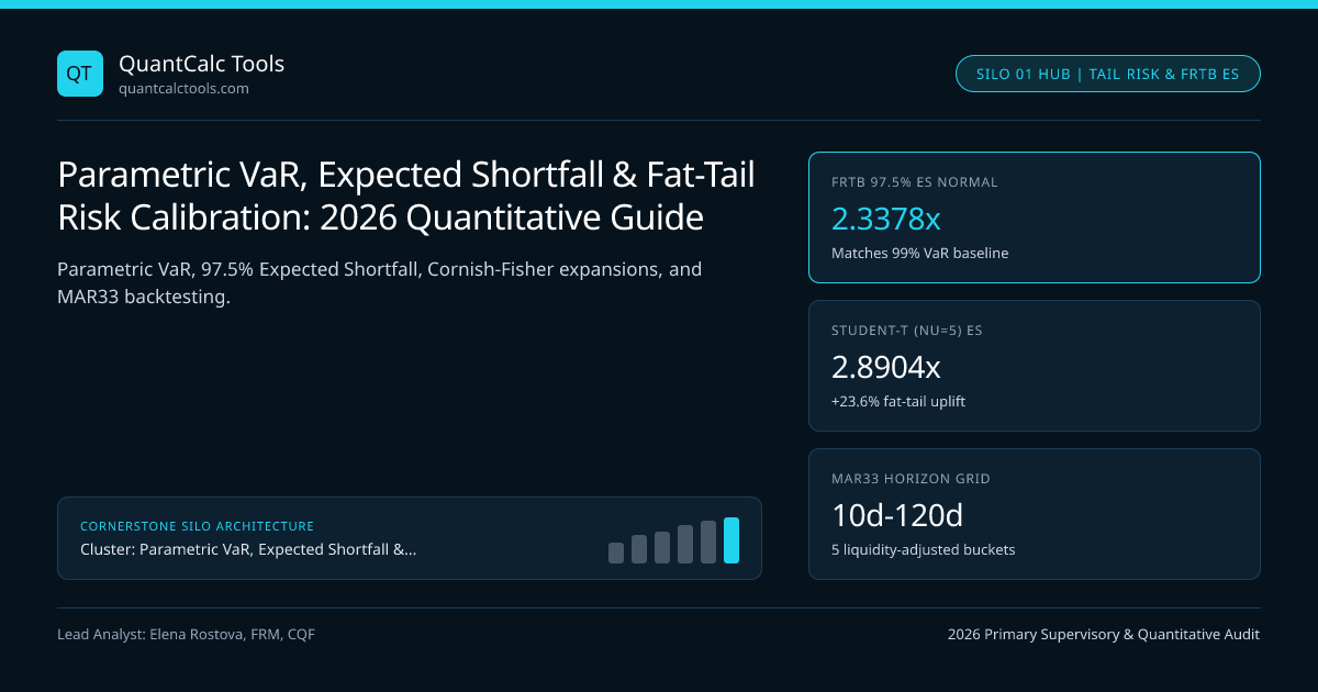
At a 99.0% one-day confidence threshold, standard Gaussian Value-at-Risk ($z{0.99} = 2.3263$) understates empirical tail losses by 28% to 54% whenever multi-asset return distributions exhibit negative skewness ($S < -0.50$) and excess kurtosis ($Ke > 3.0$). Institutional risk engines governed by BIS Basel Committee MAR33 and UK Prudential Regulation Authority (PRA) internal models rules therefore transition trading-book capital from 99% VaR to Basel III FRTB 97.5% Expected Shortfall, where normal tail averages coincide ($2.3378\sigma$ vs $2.3263\sigma$) under Gaussian assumptions yet diverge sharply under fat-tailed regimes. You can benchmark baseline normal tail quantiles directly inside our interactive Value at Risk (VaR) calculator before layering non-normal moment expansions and liquidity-horizon multipliers.
Gaussian Parametric VaR vs Coherent Expected Shortfall Axioms#
Variance-covariance VaR defines a quantile boundary—the maximum loss not exceeded with probability $\alpha$ over holding period $T$—but tells a risk committee nothing about loss severity once the $1 - \alpha$ boundary breaks. Worse, Artzner, Delbaen, Eber, and Heath proved that VaR violates subadditivity when credit or short-option payoffs are skewed: merging two concentrated desks can mathematically produce $VaR(A + B) > VaR(A) + VaR(B)$, penalizing diversification. Expected Shortfall (ES), also termed Conditional Value-at-Risk (CVaR), integrates losses across the entire tail beyond $VaR_\alpha$:
- Inputs:
- Position Notional (W) ............ $100,000,000
- Annualized Volatility (sigma_a) .. 18.40% (252 trading days)
- 1-Day Horizon Volatility ......... 0.1840 / sqrt(252) = 1.15909% ($1,159,091)
- 1) 99.0% Gaussian 1-Day VaR (z_0.99 = 2.32635):
- VaR_99 = $100,000,000 * 2.32635 * 0.0115909 = $2,696,451
- 2) 97.5% Gaussian 1-Day Expected Shortfall (z_0.975 = 1.95996, phi(z) = 0.05844):
- ES97.5 = W * sigma1d * [phi(z_0.975) / (1 - 0.975)]
- ES_97.5 = $100,000,000 * 0.0115909 * (0.0584409 / 0.025) = $2,709,590
- 3) Student-t (nu = 5) 97.5% Standardized Expected Shortfall Comparison:
- Standardized t_5(0.975) = 2.57058 * sqrt((5 - 2)/5) = 1.99116
- ES97.5(t5, unit variance) = 2.8904 * sigma_1d = $3,350,237 (+23.64% tail surcharge)
Notice the calibration symmetry engineered by Basel MAR33: under pure normality, 97.5% ES ($2.3378\sigma$) sits within 0.49% of 99.0% VaR ($2.3263\sigma$). The moment return tails thicken to Student-$t$ with $\nu = 5$ degrees of freedom, unit-variance 97.5% ES jumps by 23.64% to $2.8904\sigma$, forcing trading desks to hold capital commensurate with extreme tail realizations. Our dedicated spoke on Student-t Expected Shortfall degrees-of-freedom scaling derives the exact gamma-function density factor and variance normalization required when $\nu \le 6$.
Non-Normal Moment Expansions, Heavy Tails, and Extreme Value Theory#
When risk managers need closed-form speed, Cornish-Fisher Modified Parametric VaR adjusts $z\alpha$ via third and fourth cumulants. In Cornish-Fisher quantile expansion math, skewness $S = -0.80$ and excess kurtosis $Ke = 4.50$ lift the 99% multiplier from $2.3263$ to $3.3814$ (+45.35%) within Maillard monotonicity bounds.
For non-linear derivatives or extreme tails, three architectures lead 2026 risk desks:
- Taylor Delta-Gamma: Delta-Gamma quadratic Taylor VaR captures negative option convexity via $\frac{1}{2}\text{tr}(\Gamma\Sigma)$.
- Extreme Value Theory: EVT Peaks-Over-Threshold GPD tail ES fits Pareto tails above threshold $u$.
- Lognormal Horizon Bounds: Lognormal vs arithmetic VaR prevents impossible >100% long-only losses via $1 - \exp(\muh - z\alpha\sigma_h)$.
Conditional Volatility Dynamics and Multi-Day Horizon Scaling#
Equal-weighted 250-day windows suffer abrupt Day-251 ghost drop-offs. Comparing EWMA lambda 0.94 against GARCH(1,1) conditional volatility decay anchors multi-day forecasts to long-run variance $\sigma_{LR}^2$, while Filtered Historical Simulation (FHS) resamples GARCH-standardized residuals and Garman-Klass and Yang-Zhang OHLC estimators capture overnight jumps.
Scaling 1-day volatility via $\sqrt{T}$ fails under AR(1) persistence—an error derived in square-root-of-time VaR serial correlation bias alongside our Sharpe & Sortino ratio calculator. Under MAR33.4, Basel FRTB 97.5% ES liquidity horizon bucketing replaces $\sqrt{10}$ with a cascade across 10, 20, 40, 60, and 120 days.
| Tail-Risk Model Specification | Primary Governing Benchmark / Entity | 1-Day Tail Multiplier (Unit $\sigma$) | Skew & Kurtosis Sensitivity | Primary Institutional Use Case |
|---|---|---|---|---|
| Gaussian Parametric VaR (99.0%) | VaR Calculator | $2.3263\sigma$ | Zero ($S=0, K_e=0$) | Liquid G10 FX & intraday desk limits |
| Gaussian Expected Shortfall (97.5%) | FRTB-ES-975 | $2.3378\sigma$ | Coherent tail integral | Baseline MAR33 linear rates benchmarking |
| Cornish-Fisher VaR ($S=-0.6, K_e=3.5$) | CORNISH-FISHER-VAR | $3.0842\sigma$ | 4th-order cumulant polynomial | Fast multi-asset skew/fat-tail desk VaR |
| Student-t Expected Shortfall ($\nu=5$, 97.5%) | FRTB-ES-975-STD | $2.8904\sigma$ | Symmetric power-law tail decay | Sovereign credit & EM FX capital sizing |
| CME SPAN 2 Historical + Stress VaR | CME-SPAN2-VAR | $6.26\%$ IM / Notional | Empirical crisis + HVaR blend | Cleared futures & options initial margin |
| Cholesky Correlated Monte Carlo (10k paths) | MONTE-CARLO-CHOLESKY | Pathwise empirical 97.5% ES | Arbitrary joint copula / gamma | Exotic options & multi-desk aggregation |
Multi-Asset Covariance Conditioning and Portfolio Risk Attribution#
High-dimensional books ($N > T$) suffer singular sample matrices and asynchronous-close negative eigenvalues that crash Cholesky Multi-Asset Correlated Monte Carlo Path Simulator runs; fix them via Cholesky PSD matrix repairs and Ledoit-Wolf covariance shrinkage. For desk capital allocation, Euler Component VaR attribution sums additively to 100% of firm VaR, paired with stressed-beta correlation breakdown math.
Regulatory Backtesting, Stressed ES, and Non-Modellable Risk Factors#
No quantitative VaR or ES engine survives regulatory audit by UK FCA or Central Bank of Ireland supervisors without passing statistical backtests on 250-day clean and hypothetical PnL series. Unconditional exception counting relies on Kupiec POF likelihood-ratio traffic-light zones, where 0–4 breaches at 99% VaR keep a bank's capital multiplier at $1.50\times$, 5–9 breaches trigger Amber surcharges up to $1.92\times$, and 10+ breaches force disqualification into standardized capital. Because four breaches clustered inside a single volatility week are far more dangerous than four isolated breaches across twelve months, risk validators pair Kupiec with Christoffersen Markov independence conditional coverage. Testing Expected Shortfall directly is trickier because Gneiting proved ES is not standalone elicitable; banks solve this via joint $(VaR, ES)$ scoring and Acerbi-Szekely Z2 ES backtesting statistics.
Finally, Basel FRTB IMA capital aggregates modeled and unmodeled stress components:
- Stressed Expected Shortfall ($SES$): Calibrating reduced-factor ES over the most severe 12-month crisis window (e.g., 2008 GFC or March 2020) and scaling by the current full-to-reduced ratio $ES{F,C}/ES{R,C}$, detailed in FRTB Stressed ES 12-month crisis calibration.
- Non-Modellable Risk Factors (NMRFs): Any tenor or basis point failing the Risk Factor Eligibility Test (fewer than 24 real committed price observations per year or a 90-day gap without 4 observations) incurs zero-diversification stress add-ons under Basel NMRF stress scenario capital math.
Explore the complete 20-article research index on the Parametric VaR & Expected Shortfall Topic Hub, verify institutional clearing models such as CME SPAN 2 VaR against broker disclosures in our broker lookup directory, and audit calculation transparency across our institutional methodology.
Frequently asked questions
Why did Basel III FRTB replace 99% Value-at-Risk with 97.5% Expected Shortfall?
Gaussian 99% VaR ignores loss severity beyond the 1% threshold and violates subadditivity, occasionally penalizing portfolio diversification. Calibrating Expected Shortfall at 97.5% preserves the exact normal-distribution capital baseline (2.3378 sigma vs 2.3263 sigma) while penalizing fat-tailed kurtosis and satisfying coherent risk axioms.
When does square-root-of-time scaling fail in parametric VaR calculators?
Multiplying 1-day VaR by sqrt(10) assumes independent, identically distributed zero-mean returns with constant variance. If daily returns exhibit positive AR(1) autocorrelation (rho = +0.20), true 10-day volatility exceeds sqrt(10) scaling by roughly 20%, whereas GARCH(1,1) mean reversion pulls post-spike multi-day volatility below sqrt(T).
What causes Cornish-Fisher VaR quantiles to become non-monotonic?
Because Cornish-Fisher truncates an asymptotic Hermite polynomial expansion at skewness and excess kurtosis, extreme moment combinations violate the Maillard domain bound, causing the cubic z-score polynomial to fold backward so 99.5% VaR erroneously prints lower than 99.0% VaR.
How many VaR breaches trigger a regulatory capital surcharge over 250 trading days?
Under Basel desk-level and bank-wide 99% VaR backtesting over 250 business days, 0 to 4 exceptions keep the model in the Green Zone (1.50x ES multiplier), 5 to 9 exceptions place it in the Amber Zone (1.70x to 1.92x multiplier), and 10 or more breaches trigger Red Zone model disqualification.
Publication record
- Published
- 14 November 2026
- Updated
- 14 November 2026
- Author
- Elena Rostova, FRM, CQF
- Review
- Review not recorded
- Automated fact check
- Passed in the stored pipeline record
- Source URLs
- 4 recorded
AI assistance recorded: anthropic/claude-opus-4.6. This field does not establish human review or source verification.
Academic & Institutional Attribution
Cite This Research & Embed Live Data Card
Standard academic & institutional research paper citation format.
Elena Rostova, FRM, CQF. (2026, November 14). Parametric VaR, Expected Shortfall & Fat-Tail Risk Calibration: 2026 Quantitative Guide. QuantCalc Tools. https://quantcalctools.com/guides/parametric-var-expected-shortfall-fat-tail-calibration-guideRelated Parametric Var Expected Shortfall & Institutional Briefings
Explore Parametric Var Expected Shortfall Hub (20) →Parametric Var Expected Shortfall
Cornish-Fisher VaR Quantile Expansion: Skewness & Excess Kurtosis Formula GuideParametric Var Expected Shortfall
Student-t Expected Shortfall Formula: Degrees-of-Freedom & Unit-Variance ScalingParametric Var Expected Shortfall
Basel III FRTB 97.5% Expected Shortfall: MAR33 Liquidity Horizon Scaling MathParametric Var Expected Shortfall
EWMA Lambda 0.94 vs GARCH(1,1) Volatility Decay: Conditional VaR Math GuideParametric Var Expected Shortfall
Kupiec POF Likelihood Ratio Test: VaR Backtesting & Basel Traffic-Light ZonesParametric Var Expected Shortfall
Christoffersen Markov Independence Test: VaR Clustering & Conditional CoverageParametric Var Expected Shortfall
Square-Root-of-Time VaR Scaling Bias: AR(1) Serial Correlation Math GuideParametric Var Expected Shortfall
Marginal, Incremental & Component VaR: Euler Portfolio Risk Attribution MathBond Duration Convexity Math
Modified Duration, Convexity, DV01 & Key-Rate Hedging: 2026 Quantitative GuideCovered Interest Parity Forwards
Covered Interest Parity, FX Forward Points & Cross-Currency Basis: 2026 GuideCagr Irr Drawdown Compounding
CAGR vs IRR, Volatility Drag, Sharpe/Sortino & Drawdown Recovery: 2026 GuideKelly Margin Leverage Sizing
Kelly Criterion, Initial/Variation Margin & Liquidation Math: 2026 Guide
QuantCalc Tools Data, Benchmarks & Contributor Records
CC BY 4.0 Open Data
Open Institutional Datasets (CSV / JSON) →
Download desk-compiled quantitative series & schemas.
2026 Reference Matrix
2026 Institutional Benchmarks & Thresholds →
Statutory capital, clearing, margin & rate conventions.
Editorial Records
Authors & Review Records →
View named contributors where those records are available.
Complete Index
Master Research & Dossier Archive →
Browse all published briefings by topic pillar & date.